cost optimization

Databricks 101: An Introductory Guide on Navigating and Optimizing this Data Powerhouse

Noa Shavit
07.16.2024

In an era where data reigns supreme, the tools and platforms that businesses utilize to harness and analyze their data can make or break their competitive edge. Among these, Databricks stands out as a powerhouse, yet navigating its complexities often feels like deciphering cryptic code. With businesses generating an average of 2.5 quintillion bytes of data daily, the need for a robust, efficient, and cost-effective data cloud has never been more critical.

In this post, we demystify Databricks, with a focus on Job Clusters. Readers will gain insight into the platform’s workspace, the pivotal role of workflows, and the nuanced world of compute resources including All-Purpose Compute (APC) clusters vs Jobs Compute clusters. We’ll also shed light on how to avoid costly errors and optimize resource allocation for data workloads.

Curious about how Databricks can transform your data strategy while keeping costs in check? Read on to learn how.

Introduction to Databricks: Components and configurations

*Image source: https://www.serveradminz.com/blog/databricks-an-advanced-analytics-solution/*

Databricks, at its core, is a comprehensive platform that integrates various facets of data science and engineering, offering a seamless experience for managing and analyzing vast datasets.

Central to its ecosystem is the Workspace, a collaborative environment where data teams can store files, collaborate on notebooks, and orchestrate data workflows, to name a few capabilities. Workspaces act as the nerve center along with the Unity Catalog, which provides a bridge between workspaces. Together they facilitate an organized approach to data projects and ensure that valuable insights are never siloed.

Workflows, available under each Workspace, represent recurring production workloads (aka jobs) which are vital for database production environments. These workflows automate routine data processing tasks, such as machine-learning pipelines, ETL workloads, and data streaming, ensuring reliability and efficiency in data operations. Understanding the significance of workflows is essential for anyone looking to streamline their data processes in Databricks.

Databricks Job Clusters

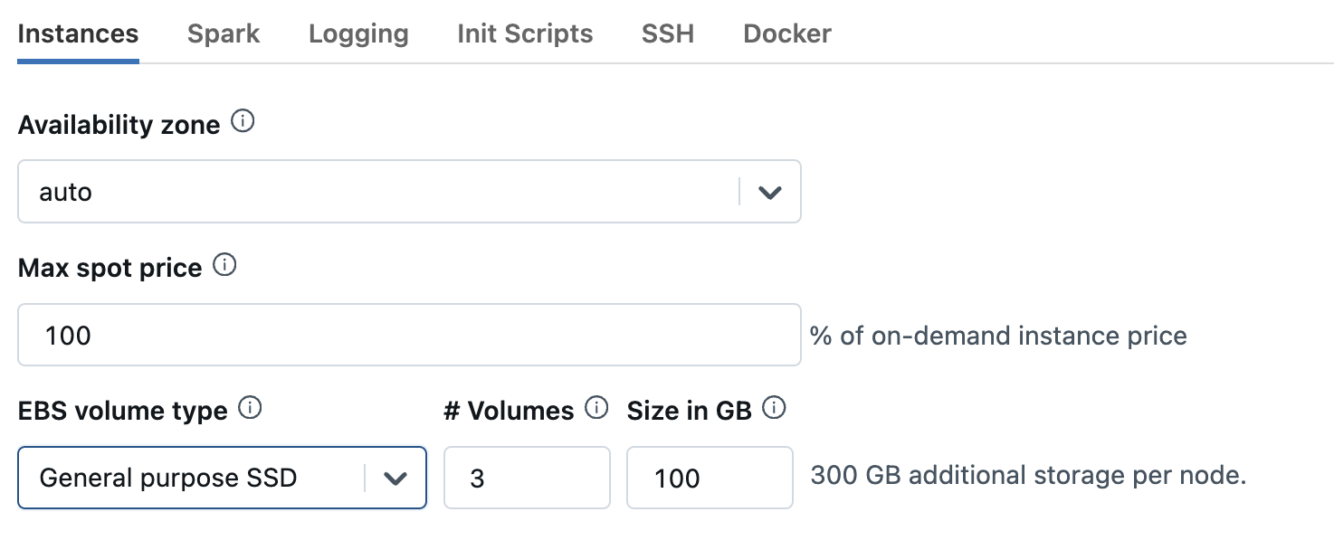
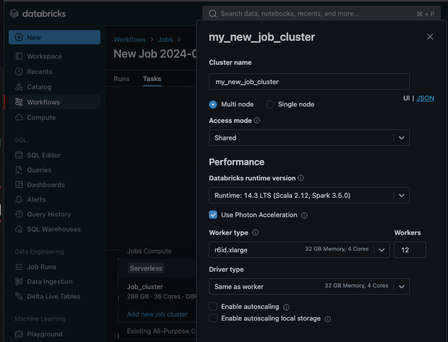
Workflows rely on Job Clusters for compute resources. Databricks offers various compute resource options to pick from during the cluster set up process. While the default cluster compute is set to Serverless, you can expose and tweak granular configuration options by picking one of the classic compute options.

Read on for more info about Databricks Job Cluster options.

Serverless Jobs vs. Classic Compute

Multiple options to pick from during the cluster set up process

Databricks recently announced the release of serverless compute across the platforms at the Data + AI 2024 conference. The goal is to provide users with a simplified cluster management experience and reduce compute costs. However, based on our research, Jobs Serverless isn’t globally cheaper than Classic Compute, and there is a price for the convenience that serverless offers.

We compared the cost and performance of serverless jobs vs jobs running on classic clusters and found that while short ad-hoc jobs are ideal candidates for serverless, optimized classic clusters outperformed their serverless counterparts by 60% in costs.

More about the lessons we learned from experimenting with Databricks Serverless Jobs.

As for the convenience aspect, it does come at a cost. Serverless compute unburdens you from setting up cluster configuration, but that also means you lose control over job performance and costs. There are no settings to tweak or prices to negotiate with cloud providers. So if you are like us, and want to be able to control the configuration of your data infrastructure this might not be the right option for you.

On-demand clusters vs. Spot instances

Compute resources form the backbone of Databricks cluster management. The basic classification of compute resources is between on-demand clusters vs Spot instances. Spot instances are considered cost effective, offering discounts of up to 90% on remnant cloud compute. However, they aren’t the most stable or reliable. This is because the number of workers running can change in the middle of a job, which is dangerous. The job runtime and cost could become highly variable, and sometimes even crash.

Overall, on-demand instances are better suited for workloads that cannot be interrupted, workloads with unknown compute requirements, and immediate launch and operation needs. Spot instances, on the other hand, are ideal for workloads that can be interrupted and stateful applications with surge usage.

Spot vs On-demand	On-demand Instances	Spot Instances
Access	Immediate	Only if there is unused compute capacity
Performance	Stable and reliable	Limited stability as workers can be pulled during a job run
Cost	Known	Varies. Up to 90% cheaper than on-demand rates
Best for	Jobs that cannot be interrupted Jobs with unknown compute requirements	Jobs that can be interrupted Stateful apps with surge usages

Spot vs On-demand Clusters

All-Purpose Compute vs Jobs Compute

Databricks offers a couple forms of compute resources, including All-Purpose Compute (APC) clusters, Jobs Compute clusters, and SQL warehouses. Each resource is designed with specific use cases in mind.

SQL warehouses, for example, allow users to query information in Databricks using the SQL programming language. APCs and Jobs Compute, on the other hand, are more general compute resources capable of running many different languages such as Python, SQL, and Scala to run your jobs. While APCs are ideal for interactive analysis and collaborative research, Jobs Compute is ideal for scheduled jobs and workflows. Understanding the distinctions and use cases for these compute resources is crucial for optimizing performance and managing costs.

Unfortunately, navigating the compute options for your clusters can be difficult. Common errors include the accidental deployment of more expensive compute resources, such as APC cluster when a Jobs Compute cluster would suffice. Such mistakes can have significant financial implications. In fact, we’ve found that APCs can cost up to 50% more than running the same job using Jobs Compute.

The difference between APC clusters and Jobs Compute clusters represents a crucial decision point for Databricks users, as they spin up a cluster. And each option is tailored to different stages of the data analysis lifecycle. Knowing these nuances can help you avoid common errors to ensure that your Databricks environment is both effective and cost-efficient. For example, APC clusters can be used for more exploratory research work while Job Clusters are used for mature production scheduled workloads.

Photon workload acceleration

Databricks Photon is a high-performance vectorized query engine that accelerates workloads.

Photon can substantially speed up job execution, particularly for SQL-based jobs and large-scale production Spark jobs. Unfortunately, Photon costs about 2x/DBU.

Learn more about the pros and cons of Databricks Photon in this post.

Many factors influence whether Photon is the right choice for you, which is why we recommend you A/B test the same job with and without Photon enabled. From our experience, 9 out of 10 organizations opt out of Photon once the results are in.

Spark autoscaling

Databricks offers an autoscaling feature to dynamically adjust the number of worker nodes in a cluster based on the workload demands.

By dynamically adjusting resources, autoscaling can reduce costs for some jobs. However, due to the spin up time cost of new workers, sometimes autoscaling can lead to increased costs. In fact, we found that simply applying autoscale across the board can lead to a 30% increase in compute costs.

Read the full analysis of Databricks autoscaling here.

Notebooks for ad-hoc research in Databricks

Databricks revolutionizes the data science and data engineering landscape with its notebook concept, which combines code with annotations. It embodies a dynamic canvas where you can breathe life into your projects.

Notebooks in Databricks excel in facilitating chunk-based code execution, a feature that significantly enhances debugging efforts and iterative development. By enabling users to execute code in segments, we eliminate the need for running entire scripts for minor adjustments. This accelerates the development cycle and promotes a more efficient debugging process.

Notebooks can run on APC clusters and Jobs Compute clusters depending on the task at hand. This choice is paramount when project requirements dictate the need for either exploratory analysis when APC is ideal, or scheduled jobs when Jobs Compute will be the most cost effective.

It’s important to note that All-Purpose Compute clusters are shared environments with a collaborative aspect. Multiple data scientists can simultaneously work on the same project with collaboration facilitated by shared compute resources. As a result, team members can contribute to and iterate on analyses in real-time. Such a shared environment streamlines research efforts, making APC clusters invaluable for projects requiring collective input and data exploration.

The journey from ad-hoc research in notebooks to the production-ready status of workflows marks a significant transition. While notebooks serve as a sandbox for exploration and development, workflows embody the structured, repeatable processes essential for production environments.

This contrast underscores the evolutionary path from exploratory analysis, where ideas and hypotheses are tested and refined, to the deployment of automated, scheduled jobs that operationalize the insights gained. It is this transition from the “playground” of notebooks to the “factory floor” of workflows that encapsulates the full spectrum of data processing within Databricks, bridging the gap between initial discovery and operational efficiency.

From development to production: Workflows and jobs

The journey from ad-hoc research in notebooks to the deployment of production-grade workflows in Databricks encapsulates a sophisticated transition, pivotal for turning exploratory analyses into automated, recurring processes that drive business operations. At the core of this transition are workflows, which serve as the backbone for scheduling and automating jobs in Databricks.

Workflows stand out by their ability to convert manual, repetitive tasks into automated sequences that run based on predefined triggers. These triggers vary widely, from the arrival of new files in a data lake to continuous data streams that require real-time processing. By leveraging workflows, data teams can ensure that their data pipelines are responsive, timely, and efficient, enabling seamless transitions from data ingestion to insight generation.

Directed Acyclic Graphs (DAGs) are central to workflows and further enhance the platform by providing a graphical representation of workflows. DAGs in Databricks allow users to visualize the sequence and dependencies of jobs, offering a clear overview of how data moves through various processing stages. This is an essential feature for optimizing and troubleshooting workflows, enabling data teams to identify bottlenecks or inefficiencies within their pipelines.

Transitioning data workloads from the exploratory realm of notebooks to the structured environment of production-grade workflows enables organizations to harness the full potential of their data, transforming raw information into actionable insights.

Orchestration and Competition: Databricks Workflows vs. Airflow and Azure Data Factory

By offering Workflows as a native orchestration tool, Databricks aims to simplify the data pipeline process, making it more accessible and manageable for its users. With that said, it also opens up a complex landscape of competition, especially when viewed against established orchestration tools like Apache Airflow and Azure Data Factory.

Comparing Databricks Workflows with Apache Airflow and Azure Data Factory reveals a compelling competitive landscape. Apache Airflow, with its open-source lineage, offers extensive customization and flexibility, drawing users who prefer a hands-on, code-centric approach to orchestration. Azure Data Factory, on the other hand, integrates deeply with other Azure services, providing a seamless experience for users already entrenched in the Microsoft ecosystem.

Databricks Workflows promise simplicity and integration, especially appealing to those who already leverage the platform. The key differentiation lies in Databricks’ ability to offer a cohesive experience, from data ingestion to analytics, within a single platform.

The strategic implications for Databricks are multifaceted. On one hand, introducing Workflows as an all-in-one solution locks users into its ecosystem. On the other hand, it challenges Databricks to continually add value beyond what users can achieve with other tools. The delicate balance between locking users in and providing unmatched value is critical; users will tolerate a certain degree of lock-in if they perceive they are receiving significant value in return.

As Databricks continues to expand its suite of tools with Workflows and beyond, the landscape of data engineering and analytics tools is set for a dynamic evolution. The balance between ecosystem lock-in and value provision will remain a critical factor in determining user adoption and loyalty. The competition between integrated solutions and specialized tools will shape the future of data orchestration, with opportunities for both consolidation and innovation.

Conclusion

In today’s data-driven world, mastering tools like Databricks is crucial. This guide aims to help simplify the management of Databricks Job Clusters. Our goal is to help you navigate the complexities and optimize resource allocation effectively.

Understanding the distinction between compute resources, such as APC clusters for interactive analysis and Jobs Compute clusters for scheduled jobs, is essential. Understanding when to apply Photon and when not to is also critical for cluster optimization. Simply choosing the right compute options for your jobs can reduce your Databricks bill by 30% or more.

The journey from exploration and research in notebooks to production-ready automated and scheduled workflows is a significant evolution. Workflows simplify data pipeline orchestration, and compete with other data orchestration tools like Apache Airflow and Azure Data Factory.

While Airflow offers extensive customization and Azure Data Factory integrates seamlessly with Microsoft services, Databricks Workflows provide a cohesive experience from data ingestion to analytics. The challenge for Databricks is to balance ecosystem lock-in with delivering unmatched value, ensuring it continues to enhance its tools and maintain user loyalty in an evolving data landscape.

If you are interested in learning more about Databricks cluster management and cost optimization follow us on Medium, or subscribe to your newsletter using the form in our footer.

If you’ve already ramped up your activity on Databricks and are looking for a way to cut costs, we can help you reduce spend by 50%. Use this free Databricks workspace health check for an estimation of your potential savings, and actionable insights into your cluster configurations (most expensive jobs, candidates for Photon and autoscaling, APC mistakes, and more).

What is Databricks Unity Catalog (and Should I Be Using It)?

Jeffrey Chou
05.29.2024

Since launching in 2013, Databricks has continuously evolved its product offerings from machine learning pipeline to end-to-end data warehousing and data intelligence platform.

While we at Sync are big fans of all things Databricks (particularly how to optimize cost and speed) we often get questions about understanding Databricks new offerings—particularly as product development has accelerated in the last 2 years.

To help in your understanding, we wrote this blog post to address the question, “What is Databricks Unity Catalog?” and whether users should be using it (the answer is yes). We walk through a precise technical answer, and then dive into the details of the catalog itself, how to enable it and frequently asked questions.

What Is the Unity Catalog in Databricks?

The Databrick’s Unity Catalog is a centralized data governance layer that allows for granular security control and managing data and metadata assets in a unified system within Databricks. Additionally, the unity catalog provides tools for access control, audits, logs and lineage.

You can think of the unity catalog as an update designed to bridge gaps in the Databrick ecosystem—specifically to eliminate and improve upon third-party catalogs and governance tools. With many cloud-specific tools being used, Databricks brought in a unified solution for data discovery and governance that would seamlessly integrate with their Lakehouse architecture. Thus, while Unity Catalog was initially billed as a governance tool, in reality it streamlines processes across the board. While simplistic, it’s not wrong to say Unity Catalog simply makes everything Databricks run smoother.

Notably, the Unity Catalog is being offered by default on the Databricks Data Intelligence Platform. This is because Databricks believes the Unity Catalog is a huge benefit to their users (and we are inclined to agree!). If you have access to the Unity Catalog, we highly recommend enabling it in your workspace.

What benefits does the Databricks Unity Catalog have to offer?

The Unity Catalog benefits can be thought of in four buckets: data governance, data discovery, data lineage, and data sharing and access.

Data Discovery

The unity catalog provides a structured way to tag, document and manage data assets and metadata. This allows for a comprehensive search interface that utilizes lineage metadata (including full lineage) history and ensures security based on user permissions.

Users can either explore data objects through the Catalog Explorer, or parse through data using SQL or Python to query datasets and create dashboard from available data objects. In Catalog explorer, users can preview sample data, read comments and check field details (50 second preview from Databricks here).

A preview of the Catalog explorer for data discovery in Unity Catalog (via Databricks/Youtube)

Data Governance

Unity Catalog is a layer over all external compute platforms and acts as a central repository for all structured and unstructured data assets (such as files, dashboards, tables, views, volumes, etc). This unified architecture allows for a governance model that includes controls, lineage, discovery, monitoring, auditing, and sharing.

Unity Catalog thus offers a single place to administer data access policies that apply across all workspaces. This allows you to simplify access management with a unified interface to define access policies on data and AI assets and consistently apply and audit these policies on any cloud or data platform.

All of Databricks governance parameters can be accessed via their Unity Catalog Governance Portal. The Databricks Data Intelligence Platform leverages AI to best understand the context of tables and columns, the volume of which can be impossible for manual categorization. This also enables you to quickly assess how many of your tables are monitored via Lakehouse Monitoring — Databricks’s new “AI for Governance tool”.

A screenshot of the Unity Catalog Governance portal shows how their Lakehouse Monitoring uses AI to automatically monitor tables and alert users to uses like PII leakage or data drift (via Databricks/Youtube)

With Lakehouse monitoring you can also set up alerts that automatically detect and correct PII leakage, data quality, data drift and more. These auto alerts are contained within their own section of the Governance Portal, which shows when the issue was first detected, and where the issue first stemmed from.

A preview of the governance action items shows how issues are identified by cause and Catalog/Schema/Table. Digging further in will reveal the time and date of first incidence as well as it where it stems from.

It incorporates a data governance framework and maintains an extensive audit log of actions performed on data stored within a Databricks account.

Data Lineage

As the importance of Data Lineage has grown, Databricks has responded with end-to-end lineages for all workloads. Lineage data includes notebooks, workflows and dashboards and is captured down to the column level. Unity Catalog users can parse and extract lineage metadata from queries and external tools using SQL or any other language enabled in their workspace, such as Python. Lineage can be visualized in the Catalog Explorer in near-real-time and

Unity Catalog’s lineage feature provides a comprehensive view of both upstream and downstream dependencies, including the data type of each field. Users can easily follow the data flow through different stages, gaining insights into the relationships between field and tables.

An example of the metadata lineage within Unity Catalog

Like their governance model, Databricks restricts access to data lineage based on the logged-in users’ privileges.

Data Sharing and Access

One of the most welcomed features of Databricks Unity Catalog is its built-in sharing method which is built on Delta Sharing, Databricks’ popular cloud-platform-agnostic open protocol for sharing data and managing permissions launched in 2021.

Within Unity Catalog you can access control mechanisms use identity federation, allowing Databricks users to be service principals, individual users, or groups. In addition, SQL-based syntax or the Databricks UI can be used to manage and control access, based on tables, rows, and columns, with the attribute level controls coming soon.

How Does Databricks Unity Catalog Enhance Data Governance and Security

Databricks has a standards-complaint security model based on ANSI SQL and allows administrators to grant permissions in their existing data lake using familiar syntax, at the level of catalogs, databases (also called schemas), tables, and views.

Unity Catalog grants user-level permissions for Governance Portal, Catalog Explorer and for data lineages and sharing. Unity Catalog in effect has one model for safeguarding appropriating access across your full data estate with permissions, row level, and column level security.
It almost allows registering and governing access to external data sources, such as cloud object storage, databases, and data lakes, through external locations and Lakehouse Federation.

Does Unity Catalog Help With Databricks Cost?

Yes, because Unity Catalog reduces both storage costs and fees for external licensing, it reduces cost compared to previous solutions. It also indirectly saves time by greatly reducing bottlenecks for ingesting data, reducing time spent on repetitive tasks by an average of 80% (according to Databricks). This all comes free and automatically enabled for all new users of the Databricks Data Intelligence Platform.

How do I set up and configure Unity Catalog in Databricks?

The following is a step-by-step guide to setting up and configuring Databricks Unity Catalog.

Confirm Your Workspace Is Enabled For Unity Catalog.
Log into your account and click Workspaces. From there check the Metastore Column. If a metastore name is preset, it means your workspace is attached to a Unity Catalog.

If your workspace doesn’t return a metastore, you’ll want to either to enable and attach your workspace, or create a Unity Catalog metastore.

Add users and assign the workspace admin role.
The user who creates a workspace is automatically added as an admin role. That admin can then add and invite users, and can assign workplace admin roles and metastore admin roles.
Create Clusters or SQL Warehouses for users to run queries and create objects. To run Unity Catalog workloads, compute resources must comply with certain security requirements. As a workspace admin, you can opt to make compute creation restricted to admins or let users create their own SQL warehouses and clusters
Grant Privileges to Users. To create objects and access them in Unity Catalog catalogs and schemas, a user must have permission to do so. See how to grant privileges and manage admin privileges.
Create New Catalogs and Schemas. To start using Unity Catalog, you must have at least one catalog defined. Catalogs are the primary unit of data isolation and organization in Unity Catalog. All schemas and tables live in catalogs, as do volumes, views, and models. You’ll want to create managed storage for the new catalog, then bind the new catalog your workspace, and then grant privileges for that catalog. Full instructions here.

What Integrations Work With Data Unity Catalog?

Unity Catalog works existing data storage systems and governance solutions such as Atlan, Fivetran, dbt or Azure data factory. It also integrates with business intelligence solutions such as Tableau, PowerBi and Qlik. This makes it simple to leverage your existing infrastructure for updated governance model, without incurring expensive migration costs (for a full list of integrations check out Databricks page here).

What if my workspace wasn’t enabled for Unity Catalog automatically?

If your workspace was not enabled for Unity Catalog automatically, an account admin or metastore admin must manually attach the workspace to a Unity Catalog metastore in the same region. If no Unity Catalog metastore exists in the region, an account admin must create one. For instructions, see Create a Unity Catalog metastore.

Unity Catalog Limitations

The following limitations apply for all object names in Unity Catalog:

Object names cannot exceed 255 characters.
The following special characters are not allowed:
- Period (.)
- Space ( )
- Forward slash (/)
- All ASCII control characters (00-1F hex)
- The DELETE character (7F hex)
Unity Catalog stores all object names as lowercase.
When referencing UC names in SQL, you must use backticks to escape names that contain special characters such as hyphens (-).

For a full list of Unity Catalog Limitations, read the full documentation for the Unity Catalog.

Unity Catalog FAQs

How does Databricks Unity Catalog differ from Hive Metastore?
Databricks Unity Catalog offers a centralized data governance model, supports external data access, data isolation, and advanced features like column-level security, while Hive Metastore has limited governance capabilities.
How Long is Lineage Data Stored in Databricks Unity Catalog?
Lineage data on Databricks Unity Catalog is retained for 1 year.
What are the supported compute and cluster access modes for Databricks Unity Catalog?
Supported access modes are Shared Access Mode and Single User Access Mode. No-Isolation Shared Mode is not supported.
What data file formats are supported for managed and external tables in Databricks Unity Catalog?
Managed tables must use the Delta table format, while external tables can use Delta, CSV, JSON, Avro, Parquet, ORC, and Text formats.
How do you enable your workspace for Databricks Unity Catalog?
You can enable Unity Catalog during workspace creation or assign an existing metastore to your workspace through the Databricks account console.
How do you control access to data and objects in Databricks Unity Catalog?
You can use admin privileges, object ownership, privilege inheritance, basic object privileges (GRANT/REVOKE), dynamic views for row/column security, and manage external locations and credentials.
What is the Databricks Unity Catalog object model?
The object model follows a hierarchical structure: Metastore ► Catalog ► Schema ► Tables, Views, Volumes, and Models.
Can you transfer ownership of objects in Unity Catalog?
Yes, you can transfer ownership of catalogs, schemas, tables, and views to other users or groups using SQL commands or the Catalog Explorer UI.
How do you create a new catalog in Unity Catalog?
You can use the CREATE CATALOG SQL command, specifying a name and managed location if needed. You must have CREATE CATALOG privileges on the metastore.
How do you grant permissions on a catalog or schema?
Use the GRANT statement with the desired privileges (e.g., CREATE SCHEMA, CREATE TABLE) and the catalog or schema name, followed by the user or group to grant access to.
What is the syntax for referring to a table in Unity Catalog?
Use the three-part naming convention: <catalog>.<schema>.<table>
How do you create a managed table in Unity Catalog?
Use the CREATE TABLE statement, specifying the table name, columns, and partitioning if needed. Managed tables are created in the managed storage location.
Can you access data in the Hive Metastore through Unity Catalog?
Yes, data in the Hive Metastore becomes a catalog called hive_metastore, and you can access tables using the hive_metastore.<schema>.<table> syntax.
How do you drop a table in Databricks Unity Catalog?
You can use the DROP TABLE statement followed by the fully qualified table name (e.g., DROP TABLE <catalog>.<schema>.<table>).

Unity Catalog is the solution to a problem was created as Databricks grew beyond its initial usage. In order to streamline the various product offerings within their ecosystem, Databricks introduced the Unity Catalog to eliminate third-party integrations, particularly in the realm of data governance. We feel this has been tremendously well executed and as Unity Catalog comes free and installed by default for all new databricks data intelligence platform users, we feel it’s highly advantageous to maximize its utility, particularly for data governance, lineage and data discovery.

Useful Links

March 2024 Release Notes

Jeffrey Chou
03.26.2024

Our team has been hard at work to deliver industry-leading features to support users in achieving optimal performance within the Databricks ecosystem. Take a look at our most recent releases below.

Worker Instance Recommendations

Introducing Worker Instance Recommendations directly from the Sync UI. With this feature, you are able to tap into optimal cluster configuration recos so that your configs are optimized for individual jobs.

The instance recos within Gradient not only optimize the number of workers, but also the worker size. For example, if you are using i3.2xl instances, Gradient will find the right instance size (such as i3.xl, i3.4xl, i3.8xl, etc) in the i3 instance type.

Instance Fleet Support

If your company is using Instance Fleet Clusters, Gradient is now compatible! There are no changes required on the user flow, as this feature is automatically supported in the backend. Just onboard your jobs like normal into Gradient, and we’ll handle the rest.

Hosted Log Collection

Running Gradient is now more streamlined than ever! You’re now able to opt into hosted log collection entirely in the Sync environment with Sync-hosted or user-hosted collection options. What does this mean? It means that there are no extra steps or external clusters needed to run Gradient, allowing Sync to do all the heavy lifting while minimizing the impact on your Databricks workspace.

With hosted DBX log collection within Gradient, you’re able to minimize onboarding errors due to annoying permission settings while increasing visibility into any potential collection failures, ultimately giving you and your team more control over your cluster log data.

Getting Started with Collection Setup
The Databricks Workspace integration flow is triggered when a user clicks on Add → Databricks Workspace after they have configured their workspace and webhook. Users will also now have a toggle option to choose between Sync-hosted (recommended) or User-hosted collection.

Sync-hosted collection – The user will be optionally prompted to share their preference for cluster logs stored for their Databricks Jobs. This will initially be an immutable setting saved on the Workspace.
- For AWS – Users will need to add a generated IAM policy and IAM Role to their AWS account. The IAM policy allows us to ec2:DescribeInstances, ec2:DescribeVolumes, and optionally an s3:GetObject and s3:ListBucket to the specific bucket and prefix to which users have configured uploading cluster logs. S3 permissions are optional because they may be using DBFS to record cluster logs. The user needs to add a “Trusted Relationship” to the IAM role to give our Sync IAM role permissions to sts:AssumeRole using an ExternalId we provide them. Gradient will then generate this policy and trust relationship for the user in a JSON format to be copy and pasted.
- For Azure – Coming soon!

User-hosted collection – For both Azure/AWS will proceed as the normal workspace integration requirements dictate

Stay up to date with the latest feature releases and updates at Sync by visiting our Product Updates documentation.

Ready to start getting the most out of your Databricks job clusters? Request a demo or reach out to us at info@synccomputing.com.

How Forma.ai improved their Databricks costs quickly and easily with Gradient

Jeffrey Chou
02.12.2024

Forma.ai is a B2B SaaS startup based in Toronto, Canada building an AI powered sales compensation system for enterprise. Specifically, they seamlessly unify the design, execution, and orchestration of sales compensation to better mobilize sales teams and optimize go-to-market performance.

Behind the scenes, Forma.ai deploys their pipelines on Databricks to process sales compensation pipelines for their customers. They process hundreds of terabytes of data per month across Databricks Jobs clusters and ad-hoc all-purpose compute clusters.

As their customer count grows, so will their data processing volumes. The cost and performance of their Databricks jobs directly impacts their cost of goods (COGs) and thus their bottom line. As a result, the efficiency of their jobs is of the utmost importance today and for their future sustainable growth.

What is their problem with Databricks?

Forma.ai came to Sync with one fundamental problem – how can they optimize their processing costs with minimal time investment? Thanks to their customer growth, their Databricks usage and costs were only increasing. They were looking for a scalable solution to help keep their clusters optimized without high overhead on the DevOps and Development teams.

Previously they had put some work into trying to optimize their jobs clusters, such as moving to different instance types for the most expensive pipelines. These pipelines and their clusters are updated frequently however, and manually reviewing configuration of every cluster regularly is simply not cost or time effective.

How Gradient Helps

Gradient provided the solution they were looking for – a way to achieve optimal clusters without the need to manually tune – freeing up their engineers to focus on building new features and accelerate development.

Furthermore, the configurations that Gradient does make are fully exposed to their engineers, so their team can actually learn and see what configurations actually matter and what the impact is. Enriching their engineers and leveling up their own Databricks experience.

Initial Results with Gradient

For a first test, Forma onboarded a real job they run in production with Gradient, enabled ‘auto-apply’ and then let Gradient control their cluster for each recurring run. After a couple cycles of learning and optimizing, the first results are shown below: an 18% cost savings and a 19% speedup without lifting a finger.

“Cost and cost control of data pipelines is always a factor, and Databricks and cloud providers generally make it really easy to spend money and pretty labor intensive to save money, which can end up meaning you spend more on the time spent optimizing than you end up saving. Gradient solves this dilemma by removing the bulk of the time spent on analysis and inspection. I’d be surprised if there was any data team on the planet that wouldn’t save money and time by using Gradient.”
Jesse Lancaster VP, Data Platform

So what did Gradient do actually?

In this first initial result, the change that had the most impact was tuning the cluster’s EBS settings (AWS only). These settings are often overlooked in favor of CPU and Memory settings.

A table of the specific parameters before and after Gradient is shown below:

	Initial Settings	Optimized Settings
ebs_volume_type	GENERAL_PURPOSE_SSD”	GENERAL_PURPOSE_SSD”
ebs_volume_count	1	4
ebs_volume_size	100	32
ebs_volume_iops	<not set>	3000
ebs_volume_throughput	<not set>	312

The initial settings reflect the typical settings Databricks provides, and is what most people use. The automatic EBS settings depend on the size of the instance chosen, with bigger instances getting more baseline storage according to AWS’s best practices. While these baseline settings are sufficient for running applications, they are often suboptimal.

We can see low level settings like IOPS and throughput are usually not set. In fact, they aren’t even available in the cluster creation Databricks console. You have to adjust these specific settings in the cluster JSON or with the Jobs API.

If you’d like to try out Gradient for your workloads, checkout the resources below:

Sync Computing Partners with Databricks for Lakehouse Job Cluster and Usage Optimization

Jeffrey Chou
02.01.2024

Self-improving machine learning algorithms provide job cluster optimization and insights for Databricks users

February 1, 2024 08:00 AM Eastern Standard Time

CAMBRIDGE, Mass. – Sync Computing, the industry-leading data infrastructure management platform built to leverage machine learning (ML) algorithms that allow users to automatically maximize data compute performance, today announced that it has joined forces with Databricks go-to-market (GTM) teams and their Technology Partner Program. The end goal is to help Databricks customers achieve lower costs, improved reliability, and automatic management of compute clusters at scale. With the collaboration of the two technology powerhouses efforts, Databricks customers will gain the opportunity to take advantage of Sync Computing’s Gradient solution for SLA optimization, real-time insights, and significant cost savings so that teams are able to focus on greater business objectives and ROI.

Platform and data engineering teams are constantly faced with changing pressures as the data infrastructure landscape becomes increasingly complex. They are met with ongoing needs to iterate quickly, gain real-time insights, and maximize performance all while managing cost. The Gradient platform by Sync Computing provides a single source of truth for cost tracking, data governance, and unified metrics monitoring.

“The management and cost of data pipelines is top of mind for engineering teams especially in the current economic climate. However, tuning clusters to hit cost and runtime goals is a task nobody has time for,” said Jeffrey Chou, CEO and co-founder of Sync Computing. “Databricks customers who use Sync’s Gradient toolkit are now open to a whole new world of opportunities as they can offload these tasks to Gradient while they focus on more urgent business goals. Organizations absolutely love the ROI they see almost immediately.”

“The collaboration between Sync and Databricks brings an entirely new perspective to code-level optimization.”

Sync Computing’s machine learning-powered optimization delivers recommendations for Databricks clusters, without making any changes at the code level. Using a closed-loop feedback system, Gradient automatically builds custom-tuned machine learning models for each Databricks job it is managing using historical run logs — continuously driving Databricks jobs cluster configurations to hit user-defined business goals.

Sync for Databricks allows companies to:

Enable platform teams full governance over config changes to meet business demands
Slash Databricks compute and operating costs by up to 50%
Gain coveted insights into DBU, cloud costs, and cluster anomalies
Hit SLAs even as data pipelines change

Sync integrates with leading cloud platforms like Amazon Web Services (AWS) and Microsoft Azure to programmatically optimize for tools like Apache Airflow and Databricks workflows, without changing a single line of code.

Learn how Sync helps organizations large and small optimize Databricks clusters at scale here.

About Sync Computing
Having been recognized as a Gartner Cool New Vendor, Sync Computing was originally spun out of MIT with the goal to make data and AI cloud infrastructure easier to control. With Sync’s one-of-a-kind solution, Gradient, users are given full ability to enable self-improving job clusters to hit SLA goals, gain infrastructure insights, and leverage tailored recommendations to achieve optimal performance. Recognized names such as Insider, Handelsblatt, Abnormal Security, Duolingo, and Adobe have relied on Sync to get the most out of the data-driven landscape with automated data optimization. To learn more, visit https://www.synccomputing.com.

Contact
McKinley Culbert
Marketing at Sync Computing
mckinley.culbert@synccomputing.com

Why Your Data Pipelines Need Closed-Loop Feedback Control

Jeffrey Chou
09.10.2023

As data teams scale up on the cloud, data platform teams need to ensure the workloads they are responsible for are meeting business objectives. At scale with dozens of data engineers building hundreds of production jobs, controlling their performance at scale is untenable for a myriad of reasons from technical to human.

The missing link today is the establishment of a closed loop feedback system that helps automatically drive pipeline infrastructure towards business goals. That was a mouthful, so let’s dive in and get more concrete about this problem.

The problem for data platform teams today

Data platform teams have to manage fundamentally distinct shareholders from management to engineers. Oftentimes these two teams have opposing goals, and platform managers can be squeezed by both ends.

Many real conversations we’ve had with platform managers and data engineers typically go like this:

“Our CEO wants me to lower cloud costs and make sure our SLAs are hit to keep our customers happy.”

Okay, so what’s the problem?

“The problem is that I can’t actually change anything directly, I need other people to help and that is the bottleneck”

So basically, platform teams find themselves handcuffed and face enormous friction when trying to actually implement improvements. Let’s zoom into the reasons why.

What’s holding back the platform team?

Data Teams are out of technical scope – Tuning clusters or complex configurations (Databricks, Snowflake) is a time consuming task where data teams would rather be focusing on actual pipelines and SQL code. Many engineers don’t have the skillset, support structure, or even know what the costs are for their jobs. Identifying and solving root cause problems is also a daunting task that gets in the way of just standing up a functional pipeline.

Too many layers of abstraction – Let’s just zoom in on one stack: Databricks runs their own version of Apache Spark, which runs on a cloud provider’s virtualized compute (AWS, Azure, GCP), with different network options, and different storage options (DBFS, S3, Blob), and by the way everything can be updated independently and randomly throughout the year. The amount of options is overwhelming and it’s impossible for platform folks to ensure everything is up to date and optimal.

Legacy code – One unfortunate reality is simply just legacy code. Oftentimes teams in a company can change, people come and go, and over time, the knowledge of any one particular job can fade away. This effect makes it even more difficult to tune or optimize a particular job.

Change is scary – There’s an innate fear to change. If a production job is flowing, do we want to risk tweaking it? The old adage comes to mind: “if it ain’t broke, don’t fix it.” Oftentimes this fear is real, if a job is not idempotent or there are other downstream effects, a botched job can cause a real headache. This creates a psychological barrier to even trying to improve job performance.

At scale there are too many jobs – Typically platform managers oversee hundreds if not thousands of production jobs. Future company growth ensures this number will only increase. Given all of the points above, even if you had a local expert, going in and tweaking jobs one at a time is simply not realistic. While this can work for a select few high priority jobs, it leaves the bulk of a company’s workloads more or less uncared for.

Clearly it’s an uphill battle for data platform teams to quickly make their systems more efficient at scale. We believe the solution is a paradigm shift in how pipelines are built. Pipelines need a closed loop control system that constantly drives a pipeline towards business goals without humans in the loop. Let’s dig in.

What does a closed loop control for a pipeline mean?

Today’s pipelines are what is known as an “open loop” system in which jobs just run without any feedback. To illustrate what I’m talking about, pictured below shows where “Job 1” just runs every day, with a cost of $50 per run. Let’s say the business goal is for that job to cost $30. Well, until somebody actually does something, that cost will remain at $50 for the foreseeable future – as seen in the cost vs. time plot.

What if instead, we had a system that actually fed back the output statistics of the job so that the next day’s deployment can be improved? It would look something like this:

What you see here is a classic feedback loop, where in this case the desired “set point” is a cost of $30. Since this job is run every day, we can take the feedback of the real cost and send it to an “update config” block that takes in the cost differential (in this case $20) and as a result apply a change in “Job 1’s configurations. For example, the “update config” block may reduce the number of nodes in the Databricks cluster.

What does this look like in production?

In reality this doesn’t happen in a single shot. The “update config” model is now responsible for tweaking the infrastructure to try to get the cost down to $30. As you can imagine, over time the system will improve and eventually hit the desired cost of $30, as shown in the image below.

This may all sound fine and dandy, but you may be scratching your head and asking “what is this magical ‘update config’ block?” Well that’s where the rubber meets the road. That block is a mathematical model that can input a numerical goal delta, and output an infrastructure configuration or maybe code change.

It’s not easy to make and will vary depending on the goal (e.g. costs vs. runtime vs. utilization). This model must fundamentally predict the impact of an infrastructure change on business goals – not an easy thing to do.

Nobody can predict the future

One subtle thing is that no “update config” model is 100% accurate. In the 4th blue dot, you can actually see that the cost goes UP at one point. This is because the model is trying to predict a change in the configurations that will lower costs, but because nothing can predict with 100% accuracy, sometimes it will be wrong locally, and as a result the cost may go up for a single run, while the system is “training.”

But, over time, we can see that the total cost does in fact go down. You can think of it as an intelligent trial and error process, since predicting the impact of configuration changes with 100% accuracy is straight up impossible.

The big “so what?” – Set any goal and go

The approach above is a general strategy and not one that is limited to just cost savings. The “set point” above is simply a goal that a data platform person puts in. It can be any kind of goal, for example runtime is a great example.

Let’s say we want a job to be under a 1 hour runtime (or SLA). We can let the system above tweak the configurations until the SLA is hit. Or what if it’s more complicated, a cost and SLA goal simultaneously? No problem at all, the system can optimize to hit your goals over many parameters. In addition to cost and runtime, other business use cases goals are:

Resource Utilization: Independent of cost and runtime, am I using the resources I have properly?
Energy Efficiency: Am I consuming the least amount of resources possible to minimize my carbon footprint?
Fault Tolerance: Is my job actually resilient to failure? Meaning do I want to over-spec it just in case I get preempted or just in case there are no SPOT instances available?
Scalability: Does my job scale? What if I have a spike in input data by 10x, will my job crash?
Latency: Are my jobs hitting my latency goals? Response time goals?

In theory, all a data platform person has to do is set goals, and then an automatic system can iteratively improve the infrastructure until the goals are hit. There are no humans in the loop, no engineers to get on board. The platform team just sets the goals they’ve received from their stakeholders. Sounds like a dream.

So far we’ve been pretty abstract. Let’s dive into a some concrete use cases that are hopefully compelling to people:

Example feature #1: Group jobs by business goals

Let’s say you’re a data platform manager and you oversee the operation of hundreds of production jobs. Right now, they all have their own cost and runtime. A simple graph below shows a cartoon example, where basically all of the jobs are randomly scattered across a cost and runtime graph.

What if you want to lower costs at scale? What if you want to change the runtime (or SLA) of many jobs at once? Right now you’d be stuck.

Now imagine if you had the closed loop control system above implemented for all of your jobs. All you’d have to do is set the high level business goals of your jobs (in this case SLA runtime requirements), and the feedback control system would do its best to find the infrastructure that accomplishes your goals. The end state will look like this:

Here we see each job’s color represents a different business goal, as defined by the SLA. The closed loop feedback control system behind the scenes changed the cluster / warehouse size, various configurations, or even adjusted entire pipelines to try to hit the SLA runtime goals at the lowest cost. Typically longer job runtimes lead to lower cost opportunities.

Example feature #2: Auto-healing jobs

As most data platform people can confirm, things are always changing in their data pipelines. Two very popular scenarios are: data size growing over time, and code changes. Both of which can cause erratic behavior when it comes to cost and runtime.

The illustration below shows the basic concept. Let’s walk through the example from left to right:

Start: Let’s say you have a job and over time the data size grows. Normally your cluster stays the same and as a result both costs and runtime increases.
Start Feedback: Over time the runtime approaches the SLA requirement and the feedback control system kicks in at the green arrow. At this point, the control system changes the cluster to stay below the red line while minimizing costs.
Code Change: At some point a developer pushes a new update to the code which causes a spike in the cost and runtime. The feedback control system kicks in and adjusts the cluster to work better with the new code change.

Hopefully these two examples explain the potential benefit of how a closed loop control pipeline can be beneficial. Of course in reality there are many details that have been left out and some design principles companies will have to adhere to. One big one is a way for configurations to revert back to a previous state in case something goes wrong. An idempotent pipeline would also be ideal here in case many iterations are needed.

Conclusion

Data pipelines are complex systems, and like any other complex system, they need feedback and control to ensure a stable performance. Not only does this help solve technical or business problems, it will dramatically help free up data platform and engineering teams to focus on actually building pipelines.

Like we mentioned before, a lot of this hinges on the performance of the “update config” block. This is the critical piece of intelligence that is needed to the success of the feedback loop. It is not trivial to build this block and is the main technical barrier today. It can be an algorithm or a machine learning model, and utilize historical data. It is the main technical component we’ve been working on over the past several years.

In our next post we’ll show an actual implementation of this system applied to Databricks Jobs, so you can believe that what we’re talking about is real!

Interested in learning more about closed loop controls for your Databricks pipelines? Reach out to Jeff Chou and the rest of the Sync Team.