As data teams scale up on the cloud, data platform teams need to ensure the workloads they are responsible for are meeting business objectives. At scale with dozens of data engineers building hundreds of production jobs, controlling their performance at scale is untenable for a myriad of reasons from technical to human.
The missing link today is the establishment of a closed loop feedback system that helps automatically drive pipeline infrastructure towards business goals. That was a mouthful, so let’s dive in and get more concrete about this problem.
The problem for data platform teams today
Data platform teams have to manage fundamentally distinct shareholders from management to engineers. Oftentimes these two teams have opposing goals, and platform managers can be squeezed by both ends.
Many real conversations we’ve had with platform managers and data engineers typically go like this:
“Our CEO wants me to lower cloud costs and make sure our SLAs are hit to keep our customers happy.”
Okay, so what’s the problem?
“The problem is that I can’t actually change anything directly, I need other people to help and that is the bottleneck”
So basically, platform teams find themselves handcuffed and face enormous friction when trying to actually implement improvements. Let’s zoom into the reasons why.
What’s holding back the platform team?
- Data Teams are out of technical scope – Tuning clusters or complex configurations (Databricks, Snowflake) is a time consuming task where data teams would rather be focusing on actual pipelines and SQL code. Many engineers don’t have the skillset, support structure, or even know what the costs are for their jobs. Identifying and solving root cause problems is also a daunting task that gets in the way of just standing up a functional pipeline.
- Too many layers of abstraction – Let’s just zoom in on one stack: Databricks runs their own version of Apache Spark, which runs on a cloud provider’s virtualized compute (AWS, Azure, GCP), with different network options, and different storage options (DBFS, S3, Blob), and by the way everything can be updated independently and randomly throughout the year. The amount of options is overwhelming and it’s impossible for platform folks to ensure everything is up to date and optimal.
- Legacy code – One unfortunate reality is simply just legacy code. Oftentimes teams in a company can change, people come and go, and over time, the knowledge of any one particular job can fade away. This effect makes it even more difficult to tune or optimize a particular job.
- Change is scary – There’s an innate fear to change. If a production job is flowing, do we want to risk tweaking it? The old adage comes to mind: “if it ain’t broke, don’t fix it.” Oftentimes this fear is real, if a job is not idempotent or there are other downstream effects, a botched job can cause a real headache. This creates a psychological barrier to even trying to improve job performance.
- At scale there are too many jobs – Typically platform managers oversee hundreds if not thousands of production jobs. Future company growth ensures this number will only increase. Given all of the points above, even if you had a local expert, going in and tweaking jobs one at a time is simply not realistic. While this can work for a select few high priority jobs, it leaves the bulk of a company’s workloads more or less uncared for.
Clearly it’s an uphill battle for data platform teams to quickly make their systems more efficient at scale. We believe the solution is a paradigm shift in how pipelines are built. Pipelines need a closed loop control system that constantly drives a pipeline towards business goals without humans in the loop. Let’s dig in.
What does a closed loop control for a pipeline mean?
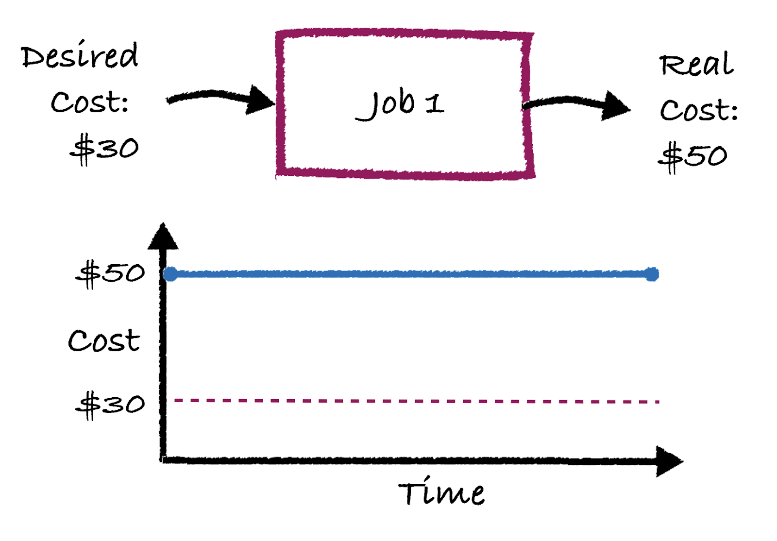
Today’s pipelines are what is known as an “open loop” system in which jobs just run without any feedback. To illustrate what I’m talking about, pictured below shows where “Job 1” just runs every day, with a cost of $50 per run. Let’s say the business goal is for that job to cost $30. Well, until somebody actually does something, that cost will remain at $50 for the foreseeable future – as seen in the cost vs. time plot.
What if instead, we had a system that actually fed back the output statistics of the job so that the next day’s deployment can be improved? It would look something like this:
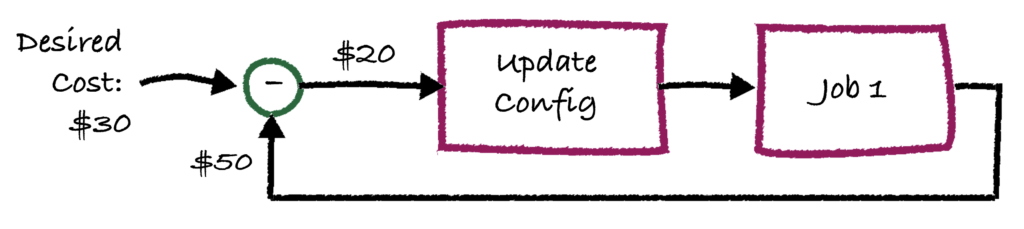
What you see here is a classic feedback loop, where in this case the desired “set point” is a cost of $30. Since this job is run every day, we can take the feedback of the real cost and send it to an “update config” block that takes in the cost differential (in this case $20) and as a result apply a change in “Job 1’s configurations. For example, the “update config” block may reduce the number of nodes in the Databricks cluster.
What does this look like in production?
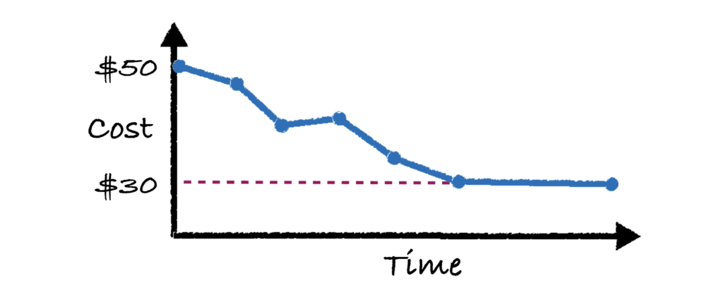
In reality this doesn’t happen in a single shot. The “update config” model is now responsible for tweaking the infrastructure to try to get the cost down to $30. As you can imagine, over time the system will improve and eventually hit the desired cost of $30, as shown in the image below.
This may all sound fine and dandy, but you may be scratching your head and asking “what is this magical ‘update config’ block?” Well that’s where the rubber meets the road. That block is a mathematical model that can input a numerical goal delta, and output an infrastructure configuration or maybe code change.
It’s not easy to make and will vary depending on the goal (e.g. costs vs. runtime vs. utilization). This model must fundamentally predict the impact of an infrastructure change on business goals – not an easy thing to do.
Nobody can predict the future
One subtle thing is that no “update config” model is 100% accurate. In the 4th blue dot, you can actually see that the cost goes UP at one point. This is because the model is trying to predict a change in the configurations that will lower costs, but because nothing can predict with 100% accuracy, sometimes it will be wrong locally, and as a result the cost may go up for a single run, while the system is “training.”
But, over time, we can see that the total cost does in fact go down. You can think of it as an intelligent trial and error process, since predicting the impact of configuration changes with 100% accuracy is straight up impossible.
The big “so what?” – Set any goal and go
The approach above is a general strategy and not one that is limited to just cost savings. The “set point” above is simply a goal that a data platform person puts in. It can be any kind of goal, for example runtime is a great example.
Let’s say we want a job to be under a 1 hour runtime (or SLA). We can let the system above tweak the configurations until the SLA is hit. Or what if it’s more complicated, a cost and SLA goal simultaneously? No problem at all, the system can optimize to hit your goals over many parameters. In addition to cost and runtime, other business use cases goals are:
- Resource Utilization: Independent of cost and runtime, am I using the resources I have properly?
- Energy Efficiency: Am I consuming the least amount of resources possible to minimize my carbon footprint?
- Fault Tolerance: Is my job actually resilient to failure? Meaning do I want to over-spec it just in case I get preempted or just in case there are no SPOT instances available?
- Scalability: Does my job scale? What if I have a spike in input data by 10x, will my job crash?
- Latency: Are my jobs hitting my latency goals? Response time goals?
In theory, all a data platform person has to do is set goals, and then an automatic system can iteratively improve the infrastructure until the goals are hit. There are no humans in the loop, no engineers to get on board. The platform team just sets the goals they’ve received from their stakeholders. Sounds like a dream.
So far we’ve been pretty abstract. Let’s dive into a some concrete use cases that are hopefully compelling to people:
Example feature #1: Group jobs by business goals
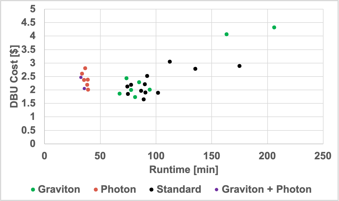
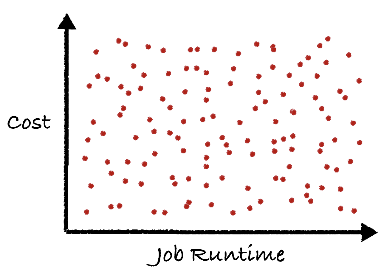
Let’s say you’re a data platform manager and you oversee the operation of hundreds of production jobs. Right now, they all have their own cost and runtime. A simple graph below shows a cartoon example, where basically all of the jobs are randomly scattered across a cost and runtime graph.
What if you want to lower costs at scale? What if you want to change the runtime (or SLA) of many jobs at once? Right now you’d be stuck.
Now imagine if you had the closed loop control system above implemented for all of your jobs. All you’d have to do is set the high level business goals of your jobs (in this case SLA runtime requirements), and the feedback control system would do its best to find the infrastructure that accomplishes your goals. The end state will look like this:
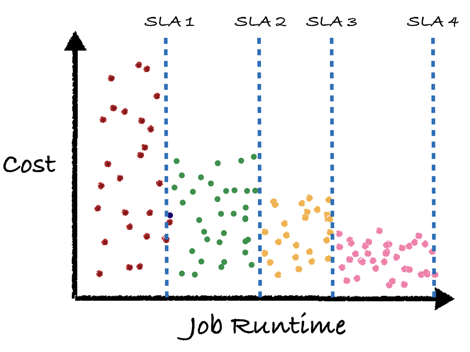
Here we see each job’s color represents a different business goal, as defined by the SLA. The closed loop feedback control system behind the scenes changed the cluster / warehouse size, various configurations, or even adjusted entire pipelines to try to hit the SLA runtime goals at the lowest cost. Typically longer job runtimes lead to lower cost opportunities.
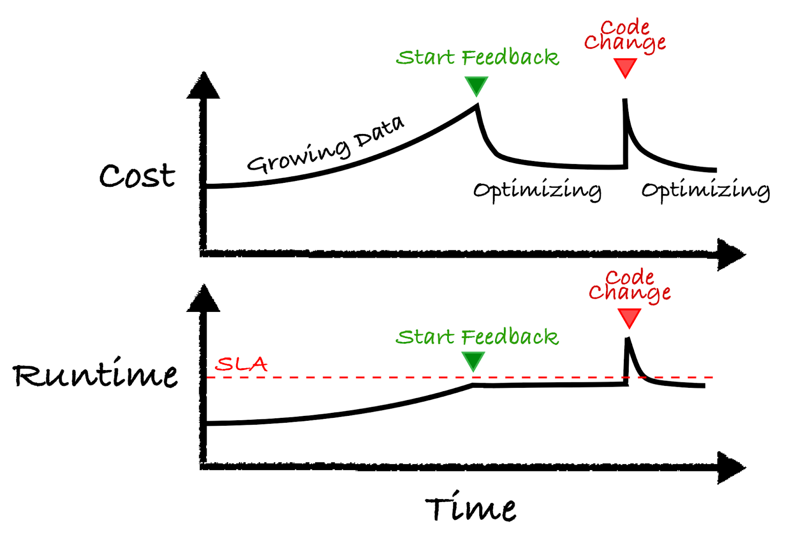
Example feature #2: Auto-healing jobs
As most data platform people can confirm, things are always changing in their data pipelines. Two very popular scenarios are: data size growing over time, and code changes. Both of which can cause erratic behavior when it comes to cost and runtime.
The illustration below shows the basic concept. Let’s walk through the example from left to right:
- Start: Let’s say you have a job and over time the data size grows. Normally your cluster stays the same and as a result both costs and runtime increases.
- Start Feedback: Over time the runtime approaches the SLA requirement and the feedback control system kicks in at the green arrow. At this point, the control system changes the cluster to stay below the red line while minimizing costs.
- Code Change: At some point a developer pushes a new update to the code which causes a spike in the cost and runtime. The feedback control system kicks in and adjusts the cluster to work better with the new code change.
Hopefully these two examples explain the potential benefit of how a closed loop control pipeline can be beneficial. Of course in reality there are many details that have been left out and some design principles companies will have to adhere to. One big one is a way for configurations to revert back to a previous state in case something goes wrong. An idempotent pipeline would also be ideal here in case many iterations are needed.
Conclusion
Data pipelines are complex systems, and like any other complex system, they need feedback and control to ensure a stable performance. Not only does this help solve technical or business problems, it will dramatically help free up data platform and engineering teams to focus on actually building pipelines.
Like we mentioned before, a lot of this hinges on the performance of the “update config” block. This is the critical piece of intelligence that is needed to the success of the feedback loop. It is not trivial to build this block and is the main technical barrier today. It can be an algorithm or a machine learning model, and utilize historical data. It is the main technical component we’ve been working on over the past several years.
In our next post we’ll show an actual implementation of this system applied to Databricks Jobs, so you can believe that what we’re talking about is real!
Interested in learning more about closed loop controls for your Databricks pipelines? Reach out to Jeff Chou and the rest of the Sync Team.