Optimize Databricks Clusters Based on Cost and Performance

A case study on how optimizing Databricks clusters can help reduce costs and accelerate runtimes

Databricks is increasingly one of the most popular platforms to run Apache Spark, as it provides a relatively friendly interface that allows data scientists to focus on the development of the analytical workloads—and efficiently build extract load transform (ELT) type operations. The multiple options it provides, by virtue of being built on top of Apache Spark, like supported languages (Java, Python, Scala, R, and SQL) and rich libraries (MLlib, graphX, sparknlp ) makes it a very attractive choice for a data compute platform.

That said, without careful consideration when creating clusters to run big data workloads, costs and runtime can easily expand beyond initial assumptions. And despite its importance, adjusting proper compute parameters is both time intensive and not immediately clear to new users.

Configuring compute infrastructure for Databricks to hit cost/performance goals can be daunting. We have been approached by many mid-sized B2B data service providers who have had the desire to improve their Databricks usage. Since their customer’s product is data, their Databricks bill and engineering time directly impacts their profit margin.

After careful investigation, we have been able to provide guidance on several workloads. Read below to see our explanation into Databricks parameters, and our case study showing how we reduced Databricks cost by increasing cluster efficiency and runtime.

First off, what are clusters in Databricks?

Databricks defines clusters as ”a set of computation resources and configurations on which you run data engineering, data science, and data analytics workloads.” In plain English this means a Databricks cluster is a combination of hardware and virtual instructions that can execute your Databricks code, referred to as your “workload”, within your Databricks workspace. They are the backbone of you get things done.

A cluster to run Databricks jobs is composed of a single driver node and possibly multiple worker nodes. Nodes themselves have hardware sucb as a CPU, memory, DISKs and cashe, used to host Spark and manage clusters. Databricks clusters can come in many forms such as notebooks (which are a set of commands) automated jobs, delta-live tables, and SQL queries. These cluster types often come in different pricing tiers.

Specific instance types must be selected for each driver or group of workers, of which there are hundreds of possible options. Selecting which cluster type to use, the pricing, cluster policies, autoscaling, and even which Databricks runtime can be a daunting task when running standard ETL pipelines.

In order to run any of those workloads, a user must first create clusters from their cloud provider, such as AWS, Microsoft Azure Databricks, or Google Cloud. Which type of cluster you create depends on everything from your data lake and Databricks runtime version to your individual workflow.

Below we go through cluster types and cluster modes and how to understand and select the type appropriate for your needs.

The Importance of Cluster Modes and Clusters Types In Databricks

When referencing clusters in Databricks, you’ll hear reference to both cluster type and cluster mode. It’s important to understand the difference to get high performance in your jobs.

There are two many cluster types: interactive (or all-purpose cluster) and job cluster.

• Interactive clusters allow you to analyze data collaboratively with interactive notebooks, and can be created using the Databricks UI via notebooks.
• Job clusters on the other hand are designed to fun fast automated workloads, such as ones using an API. Job clusters are created whenever you create a new job via CLI or Rest API. For this reason, interactive clusters can be stopped and restarted while job clusters must terminate once the job ends and cannot be restarted.

Cluster modes on the other hand refer more to the shared usage and permissions of a cluster.

• Standard clusters (now called “No Isolation Shared Access Mode”) are the defaults and can be used with Python, R, Scala and SQL. They can be shared by multiple users with no isolation between the users.
• High concurrency clusters (now called “Shared Access Mode”) are cloud-managed resources, meaning they share virtual machines across the network to provide maximum resource utilization for each notebook. This is used both for minimum query latency, as well as for users to utilize table access control, which is not supported in standard clusters. Workloads supported in these modes of clusters are in Python, SQL and R.
• Lastly, single node clusters have only one node for the driver. As the name implies, this is for a single user and in this mode, the spark job runs on the driver note itself—as there is no worker node available in this job

Standard clusters and single nodes terminate after 120 minutes by default, whereas high concurrency clusters do not. It’s important to note the mode during the cluster creation process as it cannot be changed and you must create a new cluster to update the mode.

How Optimizing Databricks Clusters Can Help Reduce Databricks Costs and Accelerate Runtimes

To that extent, a mid-sized B2B customer company that provides data services to businesses, approached Sync Computing with the desire to improve their Databricks usage. Since the customer’s product is data, their Databricks bill and engineering time directly impacts their profit margin.

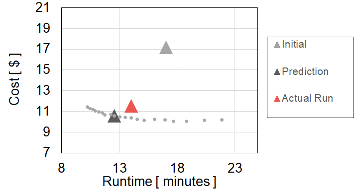
After careful investigation, we were able to provide guidance on several workloads. This particular job, after our collaboration, resulted in 34% cost reduction and 17% runtime reduction. (Though we have achieved greater gains with other Databricks jobs.) This means, we were able to not only reduce their cost but enable better capabilities around meeting their data SLAs (service level agreements).

The chart below depicts their initial cost and runtime and the associated improvements we achieved together. The gray dots represent different predictions with varying numbers of workers of the same instance type.

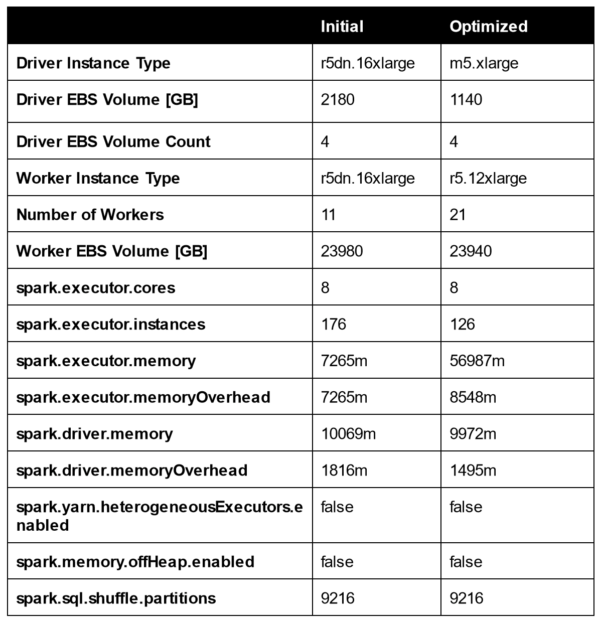
To achieve the result above, a full list of the parameters changed by Gradient is shown in table 1. By switching instance types, number of workers, memory and storage parameters all simultaneously, Gradient performs a global optimization to achieve the desired cost and performance goals selected by the user.

Out of the collaboration, several highlights may provide value to other Databricks users.  We have detailed them below (in no particular order).

Reduce Costs by Right-sizing Worker Instance Types, number of workers, and Storage

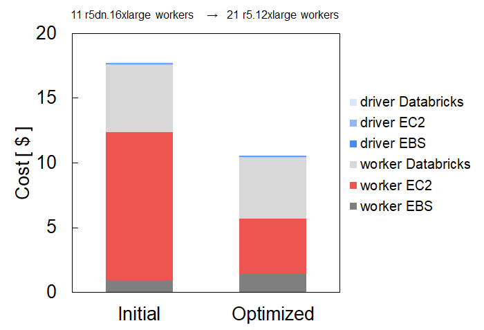
Without much insight about which instance types are worth selecting for specific workloads, it’s tempting to assemble clusters that are composed of large worker nodes with significant attached storage. This strategy is sensible for focusing not on infrastructure during development of data pipelines but once these pipelines are in production, it is worth the effort to look at cluster composition to save costs and runtime. In our collaboration with the customer, we discovered that they had the opportunity to downsize their worker node instance type, number of workers and assign appropriate storage. See figure below that illustrates this point. Our recommendation actually includes smaller worker instances and increased EBS (storage). The initial cluster included 11 r5dn.16xlarge instances and the recommended cluster included a larger number of workers (21) but smaller instance types, r5.12xlarge. The resulting cost decrease is mostly due to smaller instances despite an increase in the number. Balancing instance types and the number of workers is a delicate calculation, if done incorrectly could erase all potential gains. Gradient predicts both values simultaneously for users, to eliminate this tricky step. The costs associated with the worker EC2 instances (shown in salmon) represents where the major cost reduction occurred.  

We note that switching instances is not trivial, as it may impact other parameters. For example in this case, the r5dn instance type has attached storage. Moving to the r5 instance type requires adding the appropriate amount of EBS storage hence the small increase in the worker EBS costs. Gradient takes this into account and auto-populates the parameters such as these when suggesting to switch instance types.

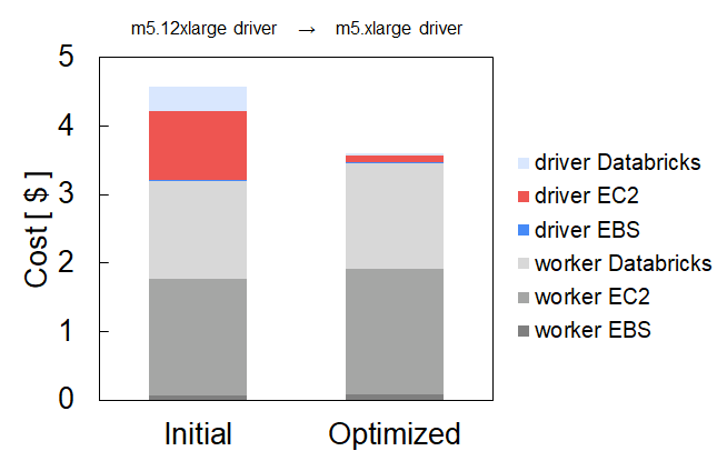
Reduce Costs by Right-sizing Driver Instance Type

Databricks provides a wide range of instance types to choose from when setting the driver and worker nodes. The plethora of options stems from the variety of compute the underlying cloud provider (AWS, Azure and GCP) put forth. The number of options can be overwhelming. A common pattern among Spark users involves choosing the same instance type for both worker and driver nodes. We have been able to help folks, like the customer, tune their cluster settings to choose more tailored driver instance types. By avoiding over-provisioning of driver nodes, the cost contribution of the driver can be reduced. This approach tends to yield strong benefits in scenarios where the driver node uses ON-DEMAND instances and the worker nodes are using SPOT instances. The benefits are more pronounced when the cluster has fewer workers.

The chart below shows the cost breakdown of a four worker node cluster. Initially, the cluster consisted of a ON-DEMAND driver m5.12xlarge instance with four SPOT m5.12xlarge workers instances. By right-sizing the driver node to a m5.xlarge instance, a 21% cost reduction is achieved. The salmon-colored portion represents the cost contribution of the change in driver instance type. The right-sizing must avoid under-provisioning so the appropriate spark configuration parameters need to be adopted. That is what the Gradient enables. A small but noticeable increase in the worker costs is related to a slight increase in the runtime associated with the driver instance change.

The impact of Spot Availability on Runtime

Using spot instances for worker nodes is a great way to save on compute costs. the customer adopted this practice prior to our initial conversations. However, the cost-saving strategy may actually result in longer runtimes due to availability issues. For large clusters, Databricks may start the job even with only a fraction of the desired total number of target worker nodes. As a result, the data processing throughput is slowly ramped up over time resulting in longer runtimes compared to the ideal case of having all the desired workers from the start. In addition, it is also possible for worker nodes to drop off, due to low Spot availability, during a run of a job and come back via Databricks Autorecovery feature. As a consequence, the total runtime for the cluster will be longer than for a cluster that has the full target number of workers for the entire job.

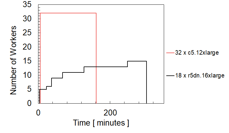
The chart below presents how Sync helped the customer accelerate their Databricks jobs by 47% by switching to a higher availability instance. The black line represents the run with up to 18 r5dn.16xlarge workers. The salmon line represents the run with 32 c5.12xlarge workers. The AWS Spot Advisor (see link) indicated that the r5dn.16xlarge instance type typically had a higher frequency of interruption, at times 10%-15% greater, than the c5.12xlarge instance type. As we see below, this small difference in interruption can lead to almost a 2x change in runtime.

The run with the c5.12xlarge workers (“low interruptibility”) had no difficulty in assembling the targeted 32 worker count from the beginning. In contrast, the run with the r5dn.16xlarge workers (“high interruptibility”) took a few minutes to start the job but with only 5 of the targeted 18 workers count. It took over 200 minutes to increase the node count to only 15 nodes, never reaching the fully requested amount of 18. Switching worker instance types also requires updates to the spark parameters (e.g. spark.executor.cores, executor memory, number of executors), fortunately Gradient adjusts these parameters as well for each instance type, making it easy for users. Gradient makes cluster configuration recommendations that take into account availability. Databricks users, like the customer, can take advantage of the cost benefits of spot instances with confidence that unforeseen availability will not negatively impact their job runtimes.

Conclusion

The compute infrastructure on which Databricks runs can have a large impact on the cost and performance of any production job. Because the cloud offers an almost endless array of compute options, understanding how to select which cloud configurations to use can lead to an intractable search space. At Sync our mission is to make this problem go away for data engineers everywhere.