databricks

Are Databricks clusters with Photon and Graviton instances worth it?

Configuring Databricks clusters can seem more like art than science.  We’ve reported in the past about ways to optimize worker and driver nodes, and how the proper selection of instances impacts a job’s cost and performance.  We’ve also discussed how autoscaling performs, and how it’s not always the most efficient choice for static jobs.  

In this blog post, we look across a few other popular questions and options we see from folks:

  1. How do Graviton instances impact cost and performance?
  2. How does the price and performance of Photon compare to standard instances?

What are Graviton instances?

Graviton instances on AWS contain custom AWS built processors, which promise to be a “major leap” in performance. Specifically for Spark, AWS published a report that claimed Graviton can help reduce costs up to 30% and speed up performance up to 15% for Apache Spark on EMR.   Although Databricks clusters can use Graviton, there haven’t been any performance metrics reported (that we know of).   There’s no extra surcharge for Graviton instances, and they are typically moderately priced compared to other instances.

What is Photon in Databricks?

Photon is a vectorized query engine written in C++ developed by the creators of Apache Spark and is available within the Databricks platform.  Photon is an amazing technical feat with a multitude of features and considerations, that extend well beyond the scope of this blog to go into.   For full details, we encourage readers to check out the original Photon academic paper here.  Unfortunately, Photon is not free and is typically a 2x cost increase for DBUs compared to non-photon.  So users have to decide if the cost increase is “worth it.”

At the highest level for most end users, as cited by the original academic paper::

  • Photon is great for CPU heavy operations such as joins, aggregations, and SQL expression evaluations.  
  • The academic paper claims about a 3x speedup on the TPC-H benchmark compared to standard Databricks runtime
  • Photon is not expected to provide a speedup to workloads that are I/O or network bound.

Yes, you can even run Photon on Graviton instances!  What happens with this powerful combo?  The data below shows the results.

How do I use Graviton and/or Photon?

Graviton instances typically have the “g” letter in the instance names, such as “m6g.xlarge” or “c7g.xlarge” and are selected during the cluster creation step within Databricks under “Worker type” and “Driver type”.

Photon is enabled by simply checking the box “Use Photon Acceleration” in the cluster creation step.  An image of the UI is shown below.

Experimental setup

In our analysis we utilize the TPC-DS 1TB benchmark, with all queries run sequentially.  We then look at the total runtime of all queries summed together.  To keep things simple and fair, every cluster has identical driver and worker instances.  We sampled 28 different instances spanning from photon enabled, Graviton, memory, compute, I/O, network, and storage optimized instances.   A full list of the parameters of each cluster are below:

  1. Driver:  [instance].xlarge
  2. Worker:  [instance].xlarge
  3. Number of workers: 10
  4. EBS volume: 64
  5. Databricks runtime version:  11.3.x-scala2.12
  6. Market:  On-demand
  7. Cloud provider: AWS
  8. Instances:  28 different instances on AWS

For the cost, we utilize only the DBU cost of each cluster.  We did not include the AWS costs for various reasons:

  • Cloud cost attribution difficulty:  Databricks internally re-uses clusters of adjacent jobs.  Meaning, AWS clusters for one job may be reused for a second job, if they require the same machine.  This causes identifying which job was using which cluster in AWS difficult to determine.  This is a niche problem, and only for people who want to determine the true cost of a single job
  • AWS costs depend on the market:  The AWS costs, or cloud costs in general, depend on the market.  Specifically, if users are using on-demand vs. spot nodes, it will drastically change the relative cost performance.  Furthermore, spot prices can fluctuate daily, so extracting fair comparisons would be difficult here.
  • AWS costs depend on contracts:  Large companies negotiate their own costs for their instances, thus again, making an overall apples to apples comparison difficult.

For the reasons above, the DBU costs are utilized because they are exact, easy to identify, and do not fluctuate depending on the market.  However, we will say that DBU costs can also depend on contracts.  But for the sake of this study, we’ll just use the list prices of DBUs.  As you can tell by these thoughts, doing actual cost comparisons is not a trivial task, and is highly dependent on each company’s use case.

Results

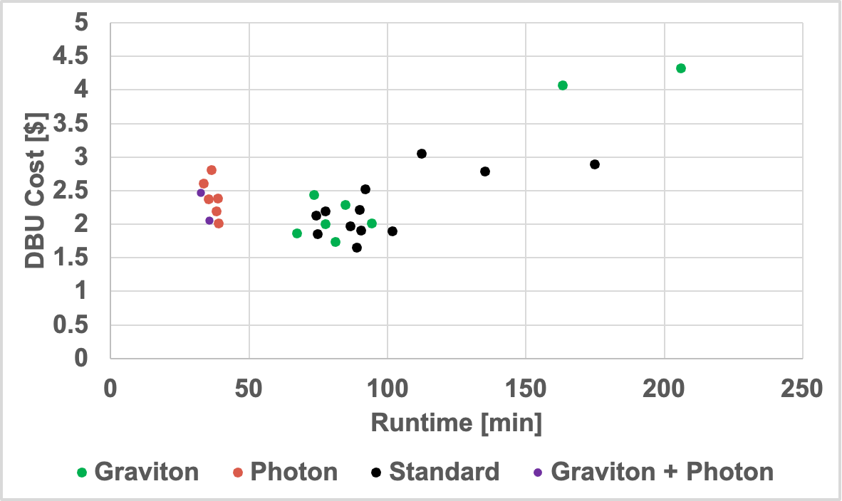
The graph below shows the cost vs runtime plots of all 28 different clusters.  They are grouped into 3 sections, “Graviton” instances, “Photon” enabled instances, “Standard” instances (no photon, no Graviton), and “Graviton + Photon” instances.  Points that are closer to the bottom left hand corner of the graph are both “faster and cheaper.”

In the graph below, we can see two clear “clusters”, basically with and without Photon.  It’s clear from this data that Photon is legitimately faster.  Unfortunately, it doesn’t appear any cheaper, so if your goal is to save money these results are a bit of a downer.  If you’re trying to run faster, Photon may be exactly what you’re looking for.

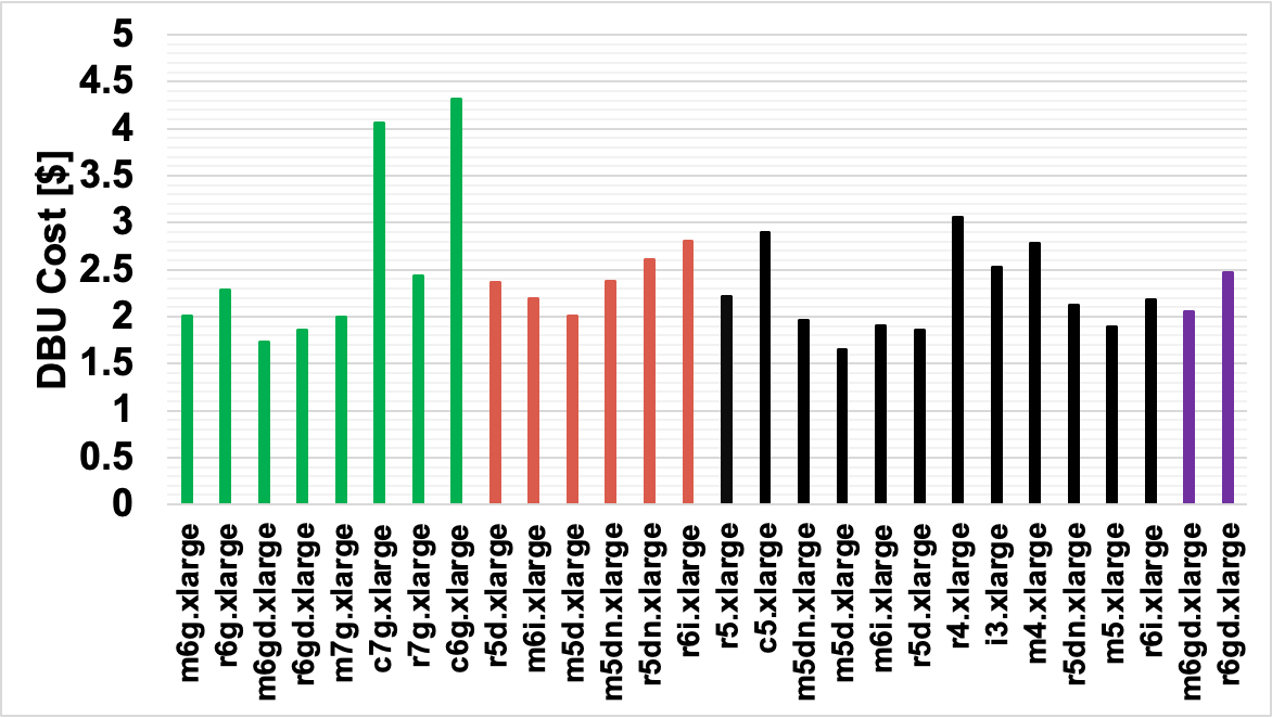
The two bar graphs below contain the same data as the XY plot above, but they break out the data into runtime and DBU costs separately.  Also, we present the individual instances used, in case people would like a more granular view into the data.

After perusing through the data, our main observations are outlined below.  I’d like to heavily caution that these observations are purely from the experiment we ran above.  We urge people to exercise caution when trying to generalize these results, as individual jobs can have wildly different results than the ones we showed above.  With that said, these are the main takeaways:

  • Photon is generally 2x faster – Across the board Photon was about 2x faster than their non-photon counterparts (same instances).  This was great to see.  Although not as high as some of the claims reported by Databricks, we understand that it is highly dependent on the workload.  In my opinion a 2x speedup is pretty impressive.
  • Graviton was neutral  – The runtime for graviton was perhaps a bit faster than standard instances, but it’s unclear if it’s statistically significant.  There doesn’t seem much risk to using Graviton, and they are newer chips so maybe they will be faster for your jobs? 
  • Photon’s total cost is cheaper (with this data) – In the data above, since the DBU costs were about the same across all 3 types, and Photon’s runtimes were about 2x faster, one can logically conclude that the cloud portion of the costs (the AWS fees) will be less with Photon.  As a result, the total cost for an end user was cheapest with Photon enabled.
  • Photon pricing makes for complex cost ROI –  Because of the previous point, determining the ROI of Photon is difficult.  It basically boils down to if the speedup is fast enough to endure the increased cost.  If it does not, then users are essentially paying more money for a potentially faster job.  If Photon speedup is fast enough, then it will be cheaper.  What that threshold is will depend on the market and any discounts.  For the sake of this study, the crossover point for on-demand instances was around 20%.  Meaning, Photon needs to be at least 20% faster than Standard to observe any cost savings.

Formula for determining Photon ROI

For those that are mathematically inclined, here is a simple formula to help determine the “speedup threshold” which is the minimum speedup Photon needs to achieve for your job in order to break even.  If your speedup is greater than this threshold, then you are saving money.

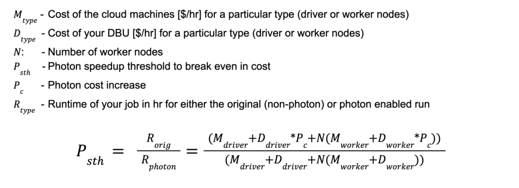
For a simple example, let’s say all of the machine and DBU costs are 1, and the Photon cost increase is a factor of 2, and we have 10 workers.  With these very simple numbers, we get a Psth value of 1.5.  Plugging in 1.5 for Psth and setting R_orig =1 and solving for R_photon, that means Photon needs to be 33% faster to break even.  Clearly this value is heavily dependent on a lot of factors, all of which are shown in the equation above.

Conclusion

Overall the answers to the original two questions really comes down to “it depends.”  The data points we showed above are an infinitely small slice of what workloads actually look like.  Based on simply the data above, here are the answers:

1)  Photon will probably be faster than non-photon, but whether or not it’s cheaper will depend on how much faster it is relative to the costs.  To understand if the 2x DBU cost increase with Photon is worth it, it all depends on the markets and pricing of your cloud instances.

2)  On average Graviton was about the same for cost and runtime compared to standard instances.  We did not see any significant advantage of using Graviton here, but we didn’t see any downside either.  Maybe these new chips will be perfect for your workload, or maybe not.  It’s hard to tell.

However, with the data above, specifically around Photon, I can’t help but ask the question:

Is Databricks motivated to make Spark run faster? 

This is an interesting philosophical question where the tech enthusiast may clash with the business units.  The faster Databricks makes Spark, the less revenue they get, since they charge per minute.  Photon is an interesting case study in which, yes, they made Spark 2x faster – but then had to double their costs to not lose money.  This is at least one data point that shows you where Databricks basically sits: “Yes we can make Spark faster, but not cheaper.”

In my opinion, Databricks, and other cloud providers, are fundamentally motivated to increase revenue.  So making Spark run faster and/or cheaper is not in alignment with where they need to do as a business.  They will however make the product easier to use, or expand to other use cases which, fundamentally, increases revenue.
We of course respect the fact that any business needs to make money, so I don’t think anything improper is happening here.  But it does reveal an interesting conflict between technology and business and how that fundamentally impacts the end user.

How to Use the Gradient CLI Tool to Optimize Databricks / EMR Programmatically

Introduction:

The Gradient Command Line Interface (CLI) is a powerful yet easy utility to automate the optimization of your Spark jobs from your terminal, command prompt, or automation scripts. 

Whether you are a Data Engineer, SysDevOps administrator, or just an Apache Spark enthusiast, knowing how to use the Gradient CLI can be incredibly beneficial as it can dramatically reduce the cost of your Spark workloads and while helping you hit your pipeline SLAs. 

If you are new to Gradient, you can learn more about it in the Sync Docs. In this tutorial, we’ll walk you through the Gradient CLI’s installation process and give you some examples of how to get started. This is meant to be a tour of the CLI’s overall capabilities. For an end to end recipe on how to integrate with Gradient take a look at our Quick Start and Integration Guides.

Pre Work

This tutorial assumes that you have already created a Gradient account and generated your

Sync API keys. If you haven’t generated your key yet, you can do so on the Accounts tab of the Gradient UI.

Step 1: Setting up your Environment

Let’s start by making sure our environment meets all the prerequisites. The Gradient CLI is actually part of the Sync Library, which requires Python v3.7 or above and which only runs on Linux/Unix based systems.

python --version

I am on a Mac and running python version 3.10, so I am good to go, but before we get started I am going to create a Python virtual environment with vEnv. This is a good practice for whenever you install any new Python tool, as it allows you to avoid conflicts between projects and makes environment management simpler. For this example, I am creating a virtual environment called gradient-cli that will reside under the ~/VirtualEnvironments path.

python -m venv ~/VirtualEnvironments/gradient-cli

Step 2: Install the Sync Library

Once you’ve confirmed that your system meets the prerequisites, it’s time to install the Sync Library. Start by activating your new virtual environment.

source ~/VirtualEnvironments/gradient-cli/bin/activate

Next use the pip package installer to install the latest version of the Sync Library.

pip install https://github.com/synccomputingcode/syncsparkpy/archive/latest.tar.gz

You can confirm that the installation was successful by viewing the CLI executable’s version by using the –version or –help options.

sync-cli --help

Step 3. Configure the Sync Library

Configuring the CLI with your credentials and preferences is the final step for the installation and setup for the Sync CLI. To do this, run the configure command:

sync-cli configure

You will be prompted for the following values:

Sync API key ID:

Sync API key secret:

Default prediction preference (performance, balanced, economy) [economy]:

Would you like to configure a Databricks workspace? [y/n]:

Databricks host (prefix with https://):

Databricks token:

Databricks AWS region name:

If you remember from the Pre Work, your Sync API key & secret are found on the Accounts tab of the Gradient UI. For this tutorial we are running on Databricks, so you will need to provide a Databricks Workspace and an Access token.


Databricks recommends that you set up a service principal for automation tasks. As noted in their docs, service principals give automated tools and scripts API-only access to Databricks resources, providing greater security than using users or groups.

These values are stored in ~/.sync/config.

Congrats! You are now ready to interact with Gradient from your terminal, command prompt, or automation scripts.

Step 4. Example Uses

Below are some tasks you can complete using the CLI. This is useful when you want to automate Gradient processes and incorporate them into larger workflows.

Projects

All Gradient recommendations are stored in Projects. Projects are associated with a single Spark job or a group of jobs running on the same cluster. Here are some useful commands you can use to manage your projects with the CLI. For an exhaustive list of commands use the –help option.

Project Commands:

create – Create a project

sync-cli projects create --description [TEXT] --job-id [Databricks Job ID] PROJECT_NAME

delete – Delete a project

sync-cli projects delete PROJECT_ID

get – Get info on a project

sync-cli projects get PROJECT_ID

list – List all projects for account

sync-cli projects list

Predictions

You can also use the CLI to manage, generate and retrieve predictions. This is useful when you want to automate the implementation of recommendations within your Databricks or EMR environments.

Prediction commands:

get – Retrieve a specific prediction

sync-cli predictions get --preference [performance|balanced|economy] PREDICTION_ID

list – List all predictions for account or project

sync-cli predictions list --platform [aws-emr|aws-databricks] --project TEXT

status – Get the status of a previously initiated prediction

sync-cli predictions status PREDICTION_ID

The CLI also provides platform specific commands to generate and retrieve predictions.

Databricks

For Databricks you can generate a recommendation for a previously completed job run with the following command:

sync-cli aws-databricks create-prediction --plan [Standard|Premium|Enterprise] --compute ['Jobs Compute'|'All Purpose Compute'] --project [Your Project ID] RUN_ID

If the run you provided was not already configured with the Gradient agent when it executed, you can still generate a recommendation but the basis metrics may be missing some time sensitive information that may no longer be available. To enable evaluation of prior logs executed without the Gradient agent, you can add the –allow-incomplete-cluster-report option. However, to avoid this issue altogether, you can implement the agent and re-run the job.

Alternatively, you can use the following command to run the job and request a recommendation with a single command:

sync-cli aws-databricks run-job --plan [Standard|Premium|Enterprise] --compute ['Jobs Compute'|'All Purpose Compute'] --project [Your Project ID] JOB_ID

This method is useful in cases when you are able to manually run your job without interfering with scheduled runs.

Finally, to implement a recommendation and run the job with the new configuration, you can issue the following command:

sync-cli aws-databricks run-prediction --preference [performance|balanced|economy] JOB_ID PREDICTION_ID

EMR

Similarly, for Spark EMR, you can generate a recommendation for a previously completed job. EMR does not have the same issue with regard to ephemeral cost data not being available, so you can request a recommendation on a previous run without the Gradient agent.

sync-cli aws-emr create-prediction --region [Your AWS Region] CLUSTER_ID

Use the following command to do so:

If you want to manually rerun the EMR job and immediately request a Gradient recommendation, use the following command:

sync-cli aws-emr record-run --region [Your AWS Region] CLUSTER_ID PROJECT

To execute the EMR job using the recommended configuration, use the following command:

sync-cli aws-emr run-prediction --region [Your AWS Region] PREDICTION_ID

Products

Gradient is constantly working on adding support for new data engineering platforms. To see which platforms are supported by your version of the CLI, you can use the following command:

sync-cli products

Configuration

Should you ever need to update your CLI configurations, you can call config again to change one or more your values.

sync-cli configure --api-key-id TEXT --api-key-secret TEXT --prediction-preference TEXT --databricks-host TEXT --databricks-token TEXT --databricks-region TEXT

Token

The Token command returns an access token that you can use against our REST API with clients like postman

sync-cli token

Conclusion

With these simple commands, you can automate the end to end optimization of all your Databricks or EMR workloads, dramatically reducing your costs and improving the performance. For more information refer to our developer docs or reach out to us at info@synccomputing.com.

Introducing: Gradient for Databricks

Wow the day is finally here! It’s been a long journey, but we’re so excited to announce our newest product: Gradient for Databricks.

Checkout our promo video here!

The quick pitch

Gradient is a new tool to help data engineers know when and how to optimize and lower their Databricks costs – without sacrificing performance.

For the math geeks out there, the name Gradient comes from the mathematical operator from vector calculus that is commonly used in optimization algorithms (e.g. gradient descent).

Over the past 18 months of development we’ve worked with data engineers around the world to understand their frustrations when trying to optimize their Databricks jobs. Some of the top pains we heard were:

  • “I have no idea how to tune Apache Spark”
  • “Tuning is annoying, I’d rather focus on development”
  • “There are too many jobs at my company. Manual tuning does not scale”
  • “But our Databricks costs are through the roof and I need help”

How did companies get here?

We’ve worked with companies around the world who absolutely love using Databricks. So how did so many companies (and their engineers) get to this efficiency pain point? At a high level, the story typically goes like this:

  • “The Honeymoon” phase: We are starting to use Databricks and the engineers love it
  • “The YOLO” phase: We need to build faster, let’s scale up ASAP. Don’t worry about efficiency.
  • “The Tantrum” phase: Uh oh. Everything on Databricks is exploding, especially our costs! Help!

So what did we do?

We wanted to attack the “Tantrum” problem head on. Internally three teams of data science, engineering, and product worked hand in hand with early design partners using our Spark Autotuner to figure out how to deliver a deeply technical solution that was also easy and intuitive. We used all the feedback on the biggest problems to build Gradient:

User Problem What Gradient Does
I don’t know when, why, or how to optimize my jobsGradient continuously monitors your clusters to notify you of when a new optimization is detected, estimate the cost/performance impact, and output a JSON configuration file to easily make the change.
I use Airflow or Databricks Workflows to orchestrate our jobs, everything I use must easily integrate.Our new python libraries and quick-start tutorials for Airflow and Databricks Workflows make it easy to integrate Gradient into your favorite orchestrators.
I just want to state my runtime requirements, and then still have my costs loweredSimply set your ideal max runtime and we’ll configure the cluster to hit your goals at the lowest possible cost.
My company wants us to use Autoscaling for our jobs clustersWhether you use auto-scaled or fixed clusters, Gradient supports optimizing both (or even switching from one to the other). 
I have hundreds of Databricks jobs. I need batch importing for optimizing to workProvide your Databricks token, and we’ll do all the heavy lifting of automatically fetching all of your qualified jobs and importing them into Gradient.

We want to hear from you!

Our early customers made Gradient what it is today, and we want to make sure it’s meeting companies’ needs. We made getting started super easy (you can Just login to the app here). Feel free to browse the docs here. Please let us know how we did via Intercom (in the docs and app).

Databricks driver sizing impact on cost and performance

As many previous blog posts have reported, tuning and optimizing the cluster configurations of Apache Spark is a notoriously difficult problem.  Especially when a data engineer needs to lower costs or accelerate runtimes on platforms such as EMR or Databricks on AWS, tuning these parameters becomes a high priority.  

Here at Sync, we will experimentally explore the impact of driver sizing in the Databricks platform on the TPC-DS 1TB benchmark, to see if we can obtain an understanding of the relationship between the driver instance size and cost/runtime of the job.

Driver node review

For those who may be less familiar with the driver node details in Apache Spark, there are many excellent previous blog posts as well as the official documentation on this topic and I will recommend users to read those if they are not familiar.  As a quick summary, the driver is an important part of the Apache Spark system and effectively acts as the “brain” of the entire operation.  

The driver program runs the main() function, creates the spark context, and schedules tasks onto the worker nodes.  Aside from these high level functions, we’d like to note that the driver node is also used in the execution of some functions, most famously when using the collect operation and broadcast joins.  During those functions, data is moved to the driver node and if it’s not appropriately sized, can cause a driver side out of memory error which can shut down the entire cluster.

As a quick side note, for broadcast joins, It looks like a ticket has been filed to change this behavior (at least for broadcast joins) in the open source Spark core.  So people should be aware that this may change in the future.

How Does Driver Sizing Impact Performance As a Function of the Number Of Workers?

The main experimental question we want to ask is “how does driver sizing impact performance as a function of the number of workers?”  The reason why we want to correlate driver size with the number of workers is that the number of workers is a very important parameter when tuning systems for either cost or runtime goals.  Observing how the driver impacts the worker scaling of the job is a key part of understanding and optimizing a cluster.

Fundamentally, the maximum number of tasks that can be executed in parallel is determined by the number of workers and executors.  Since the driver node is responsible for scheduling these tasks, we wanted to see if the number of workers changes the hardware requirements of the driver.  For example, does scheduling 1 million tasks require a different driver instance type than scheduling 10 tasks?  

Experimental Setup

The technical parameters of the experiment are below:

  • Data Platform:  Databricks
  • Compute type: Jobs (ephemeral cluster, 1 job per cluster)
  • Photon Enabled: No
  • Fixed parameters::  All worker nodes are i3.xlarge, all configs default
  • Sweep parameters:  Driver instance size (r5a.large, r5a.xlarge, r5a.4xlarge), number of workers
  • AWS market:  On-demand (to eliminate spot fluctuations)
  • Workload: Databrick’s own benchmark on  TPC-DS 1TB (all queries run sequentially)

For reference, here are the hardware specifications of the 3 different drivers used on AWS:

The result

We will break down the results into 3 main plots.  The first is below where we look at runtime vs. number of workers for the 3 different driver types.  In the plot below we see that as the number of workers increases the runtime decreases.  We note here that the scaling trend is not linear and there is a typical “elbow” scaling that occurs.  We published previously the general concept of scaling jobs.  We observe here that the largest driver, r5a.4xlarge, yielded the fastest performance across all worker sizes.

In the plot below we see the cost (DBU’s in $) vs. number of workers.  For the most part we see that the medium sized driver, r5a.xlarge is the most economical, except for the smallest number of workers where the smallest driver size r5a.large was the cheapest.

Putting both plots together, we can see the general summary when we plot cost vs. runtime.  The small numbers next to each point show the number of workers.  In general, the ideal points should be toward the bottom left, as that indicates a configuration that is both faster and cheaper.  Points that are higher up or to the right are more expensive and slower.  

Some companies are only concerned about service level agreement (SLA) timelines, and do not actually need the “fastest” possible runtime.  A more useful way to think about the plot below is to ask the question “what is the maximum time you want to spend running this job?”  Once that number is known, you can then select the configuration with the cheapest cost that matches your SLA.  

For example, consider the SLA scenarios below:

1)  SLA of 2500s – If you need your job to be completed in 2,500s or less, then you should select the r5a.4xlarge driver with a worker size of 50.

2)  SLA of 4000s – If you need your job to be completed in 4,000s or less, then you should select the r5a.xlarge driver with a worker size of 20.

3)  SLA of 10,000s – If you need your job to be completed in 10,000s or less, then you should select the r5a.large driver with a worker size of 5.

Key Insights

It’s very convenient to see the scaling trend of all 3 drivers plotted in this manner, as there are several key insights gained here:

  1. There is a general “good” optimal driver for TPC-DS 1TB – across the spectrum, it’s clear that r5a.xlarge is a good choice generally as it is usually cheaper and faster than the other driver sizes.  This shows the danger that if your driver is too big or too small, you could be wasting money and time.  
  2. At the extremes, driver size matters for TPC-DS 1TB  – At the wings of either large clusters (50 workers) or small clusters (5 workers) we can see that the best driver selection can swing between all 3 drivers.  
  3. Drivers can be too big – At 12 workers, the r5a.4xlarge performance is slightly faster but significantly more expensive than the other two driver types.  Unless that slight speedup is important, it’s clear to see that if a driver is too large, then the extra cost of the larger driver is not worth the slight speedup.  It’s like buying a Ferrari to just sit in traffic – definitely not worth it (although you will look cool).
  4. Small driver bottleneck – For the small driver curve (r5a.large), we see that the blue line’s elbow occurs at a higher runtime than the middle driver (r5a.xlarge).  This implies that the smaller driver is creating a runtime bottleneck for the entire workload as the cluster becomes larger.  The next section will dive into why.

Root cause analysis for the “small driver bottleneck”

To investigate the cause of the small driver bottleneck, we looked into the Spark eventlogs to see what values changed as we scaled the number of workers.  In the Spark UI in Databricks, the typical high level metrics for each task are shown below and plotted graphically.  The image below shows an example of a single task broken down into the 7 main metrics:

When we aggregated all of these values across all tasks, across all the different drivers and workers, the numbers were all pretty consistent, except for one number:  “Scheduler Delay”.   For those who may not be familiar, the formal definition from the Databricks Spark UI, is shown in the image below:

“Scheduler delay includes time to ship the task from the scheduler to the executor, and time to send the task result from the executor to the scheduler. If scheduler delay is large, consider decreasing the size of tasks or decreasing the size of task results.”

In the graph below, we plot the total aggregated scheduler delays of all tasks for each of the job configurations vs the number of workers.  It is expected that the aggregated scheduler delay should increase for a larger number of workers since there are more tasks.  For example, if there are 100 tasks, each with 1s of scheduler delay, the total aggregated scheduler day is 100s (even if all 100 tasks executed in parallel and the “wall clock” scheduler delay is only 1s).  Therefore, if there are 1000 tasks, the total aggregated scheduler should increase as well.  

Theoretically this should scale roughly linearly with the number of workers for a “healthy” system.  For the “middle” and “large” sized drivers (r5a.xlarge and r5a.4xlarge respectively), we see the expected growth of the scheduler delay.  However, for the “small” r5a.large driver, we see a very non-linear growth of the total aggregated scheduler delay, which contributes to the overall longer job runtime.  This appears to be a large contributor to the “small driver bottleneck” issue.

To understand a bit deeper as to what is the formal definition of Scheduler Delay, let’s look at the Spark source code inside the function AppStatusUtils.scala.  At a high level, scheduler delay is a simple calculation as shown in the code below:

schedulerDelay = duration – runTime – deserializeTime – serlializeTime – gettingResultTime

To put it in normal text, scheduler delay is basically a catch-all term, that is the time the task is spent doing something that is not executing, serializing data, or getting results.  A further question would be to see which one of these terms is increasing or decreasing due to the smaller driver?  Maybe duration is increasing, or maybe gettingResultTime is decreasing?  

If we look at the apples to apples case of 32 workers for the “medium” r5a.xlarge driver and the “small” r5a.large driver, the runtime of the “small” driver was significantly longer.  One could hypothesize that the average duration per task is longer (vs. one of the other terms becoming smaller).  

In summary, our hypothesis here is that by reducing the driver size (number of VCPUs and memory), we are incurring an additional time “tax” on each task by taking, on average, slightly longer to ship a task from the scheduler on the driver to each executor.  

A simple analogy here is, imagine you’re sitting in bumper to bumper traffic on a highway, and then all of a sudden every car (a task in Spark) just grew 20% longer, if there are enough cars you could be set back miles.

Conclusion

Based on the data described above, the answer to the question above is that inappropriately sized drivers can lead to excess cost and performance as workers scale up and down.  We present a hypothesis that a driver that is “too small” with too few VCPUs and memory, could cause, on average, an increase in the task duration via an additional overhead in the scheduler delay.  

This final conclusion is not terribly new to those familiar with Spark, but we hope seeing actual data can help create a quantitative understanding on the impact of driver sizing.  There are of course many other things that could cause a poor driver to elongate or even crash a job, (as described earlier via the OOM errors).  This analysis was just a deep dive into one observation.

I’d like to put a large caveat here that this analysis was specific to the TPC-DS workload, and it would be difficult to generalize these findings across all workloads.  Although the TPC-DS benchmark is a collection of very common SQL queries, in reality individual code, or things like user defined functions, could throw these conclusions out the window.  The only way to know for sure about your workloads is to run some driver sizing experiments.

As we’ve mentioned many times before, distributed computing is complicated, and optimizing your cluster for your job needs to be done on an individual basis.  Which is why we built the Apache Spark Autotuner for EMR and Databricks on AWS to help data engineers quickly find the answers they are looking for.