How to evaluate the performance of your Databricks Jobs clusters with Gradient

We present real user case studies of evaluating the ROI of Gradient for Databricks jobs clusters and explain the complexities of the analysis

Many data engineers and platform managers at companies want to understand “How are my pipelines doing from a cost and performance perspective?”

It turns out this very benign and simple question is riddled in complexity.  Fundamentally there are so many things that can change from run to run, that even determining if it’s the same job can be tricky to determine.

Here at Sync we literally battle this question every day, and have seen a wide variety of use cases that can make this seemingly simple analysis a complex nightmare.  

The first step when evaluating your pipelines, is to make sure you’re comparing apples to apples.  For example, a user can look at the cost of a pipeline today vs. last week and see a huge uptick in cost.  

What happened between last week and this week?  Is something really inefficient or did something else change?  How do I know if this is “normal” or actually an anomaly?  Am I really comparing the same pipeline here?

What can change?

At Sync we’ve monitored and optimized millions of core hours and have seen so many ways cluster performance can change.  The top 5 common reasons are listed below:

1. Data size can change regularly
2. Data size can change randomly
3. Code changes 
4. Spot to On-Demand market changes
5. SLA requirements changes

With all of the lessons learned with Gradient, we summarize the main metrics we look at for our users in a comprehensive summary table that can quickly tell the narrative of the performance of your clusters.

In the table we list the metrics below:

• Average Cost – The average cost of a single job run based on N samples
• Average Runtime – The average runtime of a single job based on N samples
• Average Data Size – The average input data size of a single job based on N samples
• Average cost per GB – The Average Cost / Average Data Size 
• SLA – The % of times the job runtime fell below the desired SLA during the N samples
• Market Breakdown – The % breakdown of the job clusters belonging to either spot or on-demand market (this is due to Databrick’s “spot with fallback” option)

With those metrics, a user can quickly get a glance into what changed with the job in terms of cost and performance, and whether or not we’re actually comparing apples to apples.

Across the parameters above we want to compare two states to determine the change in the cluster performance, the “Starting” and “Current” cluster performance metrics. 

• “Starting” is the case before Gradient has done any optimization and showcases the baseline values. 

• “Current” is where the cluster is at today, after Gradient has optimized the cluster.  

For both states, they can consist of many sample points, since the same configuration can be applied for many runs.  For example, we may collect 100 “starting” baseline runs with initial user selected configurations, and “current” may consist of 40 runs with the latest configuration from Gradient.

Below are a few case studies from real user jobs managed by Gradient (not fake results, nor results generated by our own internal test jobs).  We’ll see that depending on the values within the table, the narrative on the ROI of Gradient can vary quite a bit.

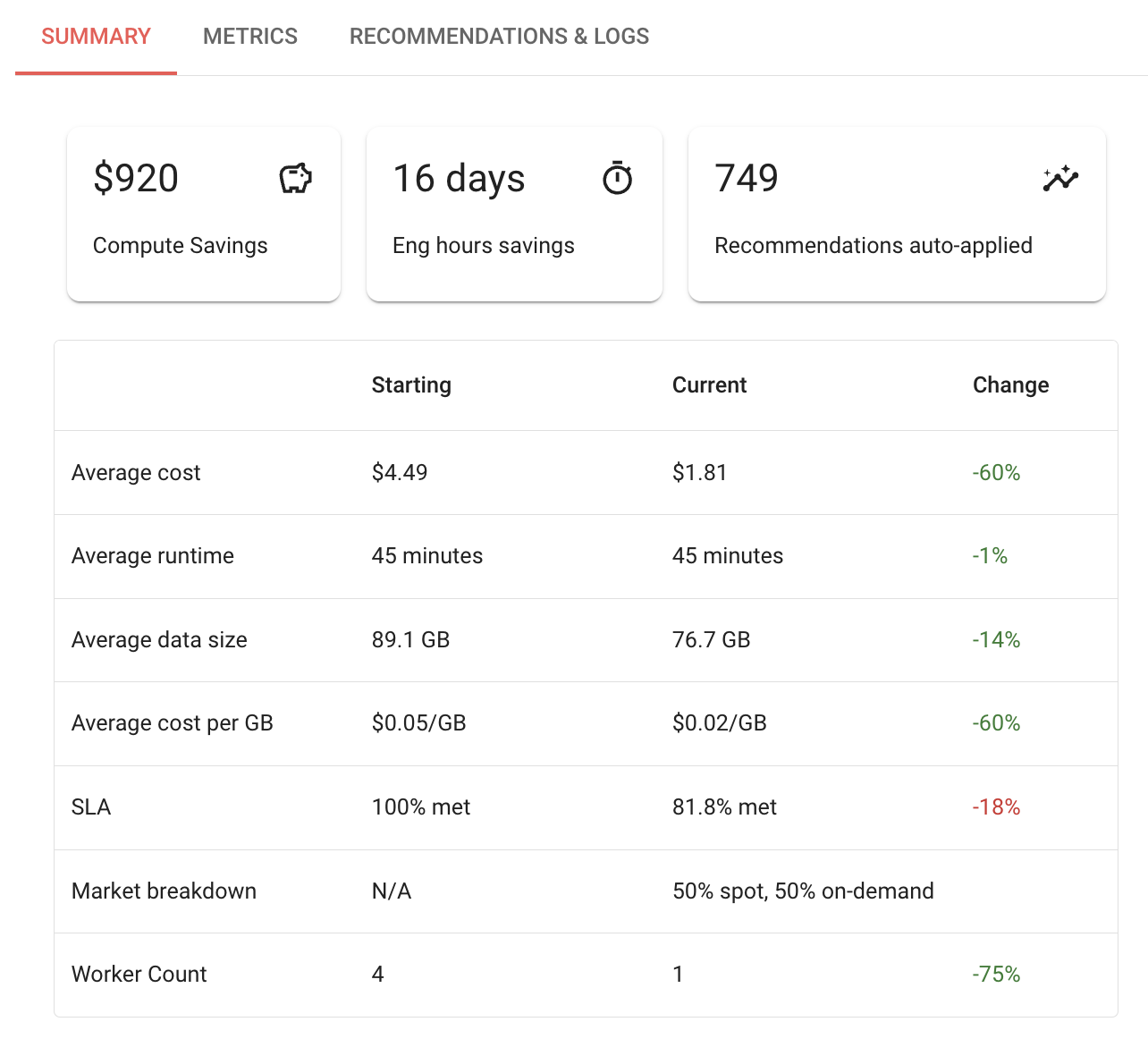
Case #1 – Clear and easy cost improvement

In this particular case, there’s a lot of green in the change column.  The average cost decreased by 60%, data size was about the same (decreased only by 14%), and the cost per GB also went down by 60%.  It’s pretty clear here that Gradient was able to make a substantial improvement to the cost of the cluster.

We do see that the SLA met went down by 18%, which may or may not be meaningful to users depending on their SLA tolerance.  In this case, the 60% cost reduction may be “worth it.”

Here’s another clear cut example, where the data size was about the same, while the costs went down by over 50%.  What’s interesting here, is that the “current” markets were more on-demand than the starting clusters, which usually means costs will go up.

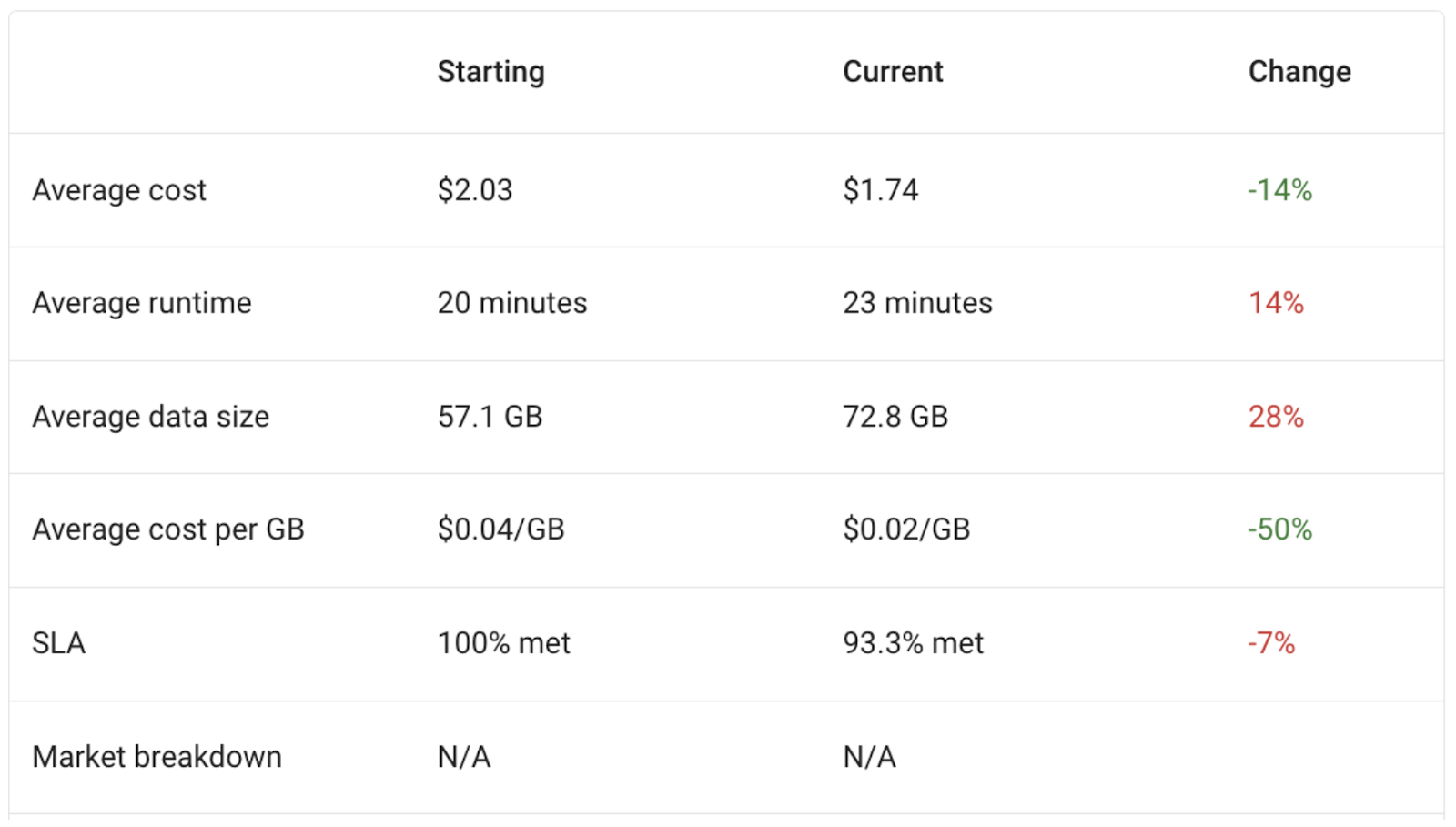
Case #2 – Data size grew, but $/GB improved a lot

The screen shot below is a very popular case we observe where the costs may grow or decrease slightly, but the $/GB improves dramatically.  In this case we see that the data size grew by 28%, which normally means the jobs will run about 28% longer (and hence cost about 28% more).

However, Gradient was able to adjust the cluster for the data size and still reduce costs.  In this case, we feel the fair metric is to look at the $/GB metric, which shows a huge improvement of 50%.

The ability for Gradient to optimize the cluster despite fluctuations in data size is a huge value add for data engineers.

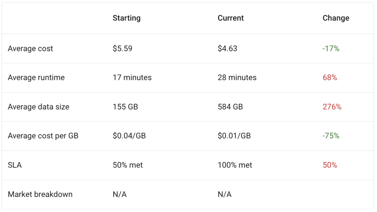
Here’s another user’s job with a similar narrative, where the data size grew by a whopping 276%, but the average $/GB dropped by 75%.  The absolute average cost only dropped by 17%.

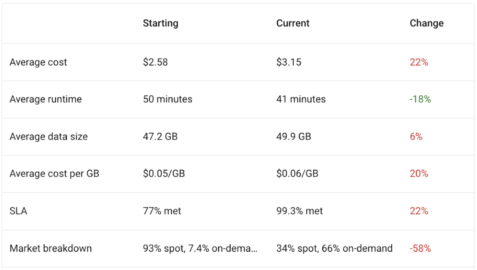
Case #3 – Costs increased, but the market comparison isn’t the same

Below is a case we sometimes see where all of the costs have increased.  This may initially look like a very bad case, but in reality it’s simply a reflection of the cluster market.

In the “Market breakdown” row, we see that the starting clusters were mostly spot clusters, which are typically about 2x cheaper than on-demand).  The current clusters were mostly on-demand, which resulted in a higher cost.

So we can attribute the cost increase as simply a mismatch in the market comparison.  It’s not fair to compare a cluster cost with all spot to and all on-demand cluster, since there’s a clear cost difference here.

In this scenario – we need more data points to make sure we can compare similar market compositions.  Soon in Gradient, we’ll make it easy to just down select specific markets to do a quick fair comparison.

One note, is in this case the SLA % met improved by 22%, so perhaps that is the metric most concerning to this user.

Case #4 – SLA % improvement, but costs went up

In this case we can see that the total cost went up dramatically, by almost 70%.  However, for this user the goal was to hit an aggressive SLA of about 1 hour (from 2 hours).  We can see in the “average runtime” row, the runtime did improve by 41% to hit the required SLA.

Since in this case getting close to the SLA was the primary goal over costs, we can still claim “mission accomplished” here.  

Although many users look for cost savings, Gradient actually can also help achieve SLAs, which may result in higher costs.  

Conclusion

We hope these real user case studies help to illuminate the complexity and subtleties of cluster optimization.  Many people may think it’s just about looking at the costs from “before” and “after” and seeing if things went down.  Or maybe people think it’s as simple as just “reducing the cluster size” to lower costs.

The reality is that changes in data size, code changes, and market composition make the problem of managing clusters a continuous and stochastic process.  Our solution, Gradient, continuously monitors and adapts the clusters for optimal performance using our advanced machine learning models which can compensate for all of these random variations.

Although costs are a very popular concern, Gradient goes beyond just cost savings and helps manage clusters by allowing users to simply declare their desired performance goals.

Try Gradient out for yourself to manage your Databricks jobs clusters for free!  Feel free to reach out to us to schedule a live demo with our team.