How Duolingo reduced their EMR job cost by 55%

See how Sync cut Duolingo’s ETL and ML costs in half.

Launch to the cloud based on cost and time: This article explains Sync Computing’s Spark Cluster Gradient Solution and how it was used to reduce Duolingo’s AWS EMR Spark costs by up to 55%. This solution eliminates the inefficient manual tuning and guesswork currently used when configuring Spark clusters and settings to provide the best cost, performance, and reliability — without any code changes.

The Problem with Spark Infrastructure

Determining cloud infrastructure settings to optimize job cost and speed for modern Spark jobs is neither practical nor possible for cloud developers. Even with optimal settings for one job, Spark jobs vary daily in code base, data sizes, and cloud spot pricing resulting in wide variations of cost/performance to developers. Most cloud users rely on simple rules of thumb or recommendations from co-workers or past jobs on what settings should be selected. Optimizing these choices requires sweeping through instance types, cloud settings, and spark configurations, a task no busy data engineer has time for.

What if it were possible to explore the effects of hardware changes without having to actually rerun jobs? Buried within the output of every Spark run is a trove of information connecting its performance to the underlying hardware. When combined with deep mathematical modeling, this data can be used to predict application performance on different cloud hardware configurations. This is the core idea behind Sync’s first solution, the Spark Cluster Gradient.

How Sync Spark Cluster Gradient can Help

Sync’s Spark Cluster Gradient removes the burden of choosing the right AWS cluster hardware and spark configurations for your recurring production Spark applications. Using only your most recent Spark eventlog and its associated cluster information, the Cluster Gradient returns the optimal cluster and spark configurations for your next run.

Whether “optimal” to you means the fastest, cheapest, or somewhere in between, the Cluster Gradient will give you the appropriate settings for your needs.

Figure 1: Example configuration selections from the Spark Cluster Gradient. These options are presented to a user within minutes of uploading a Spark eventlog.

How Sync Spark Cluster Gradient works

The Cluster Gradient works by mathematically modeling the task-level details of a spark eventlog and calculating how those details will change on different hardware configurations, resulting in an estimate of the runtime on each set of hardware.

Runtime estimates are combined with the latest AWS pricing and reliability information to yield performance estimates (runtime and cost) for each configuration. An optimization calculation is performed to search through all the configurations to pick the best options for the user.

Figure 2: Basic workflow of the Spark Predictor

Duolingo’s Situation

Duolingo builds the world’s #1 language learning application serving over 40 million monthly active users. As a cloud native company, Duolingo processes terabytes of data daily on the cloud, leading to exorbitant costs. Utilizing the cloud efficiently directly impacts the company’s bottom line.

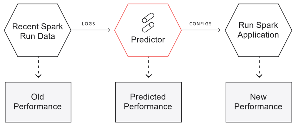
In the following section, we demonstrate a case study of this solution’s use with Duolingo. The experiment follows the workflow depicted in Figure 2.

Duolingo has a number of recurring production Spark jobs run on AWS EMR, which when run daily or even multiple times per day, incur substantial costs over the course of a year. Their #1 priority was to reduce costs, even at the expense of runtime. Figuring out the best configuration on their own would require extensive manual testing and parameter sweeps, a many-hour task no engineer has the bandwidth for.

Sync presented them with the Spark Cluster Gradient, which would get rid of manual experimenting, to instantly reduce their cloud costs on two of their ETL jobs. Basic information of these jobs is outlined in Table 1.

Job	Input Runtime (min)	Input Data Size (TB)	Input Cost ($)
ETL-D	18	2	6
ETL-P	113	5	101

Table 1

The most recent eventlog from each job was run through the Cluster Gradient and the configurations which yielded the lower cluster costs were used in the subsequent runs. The results of this experiment are depicted in Figure 3. For both jobs, the Sync Optimized configuration resulted in a substantial reduction in cost, without touching any code for an easy and fully reversible demonstration.

Figure 3: Cost efficiency of three Spark jobs before and after using the Sync Spark Cluster Gradient

The Prediction

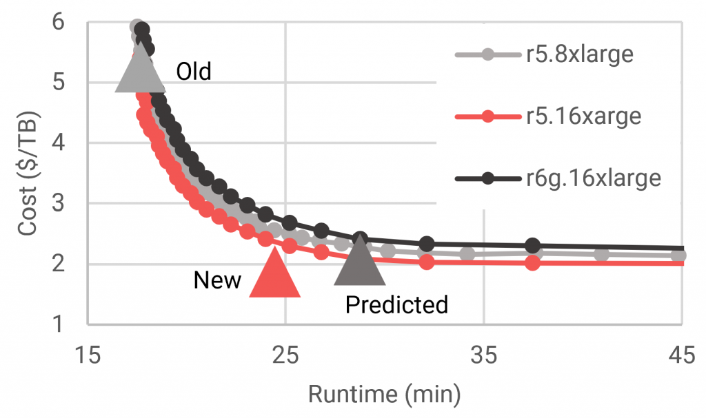
Figure 4 shows a subset of the predictions using Duolingo’s ETL-D log. Three instance types are shown, where each point on the respective curve represents a different number of workers. Performance estimates of the input, predicted, and measured jobs are indicated by the red, green, and blue triangles, respectively.

Figure 4: Performance predictions on varying hardware configurations for the ETL-D job. The performance points of the input, prediction, and measurement are indicated by the triangles.

In this example, a small number of workers in the prediction results in long-running but inexpensive jobs. As the number of workers increases, the application is expected to be faster but costlier. The initial input configuration was deep in the plateau of diminishing returns of cluster scaling. The recommendation was therefore to reduce the number of workers in order to move away from the runtime plateau.

The key insight enabled by the Cluster Gradient is given by the knowledge of where your current job lies on the performance curve, and what you need to change to get to another point on that curve. In Duolingo’s case, cost was the only relevant parameter. On the other hand, if runtime was a critical parameter, then it would be easy to pick another point on this curve that runs nearly as fast as the original job but still with significant cost savings.

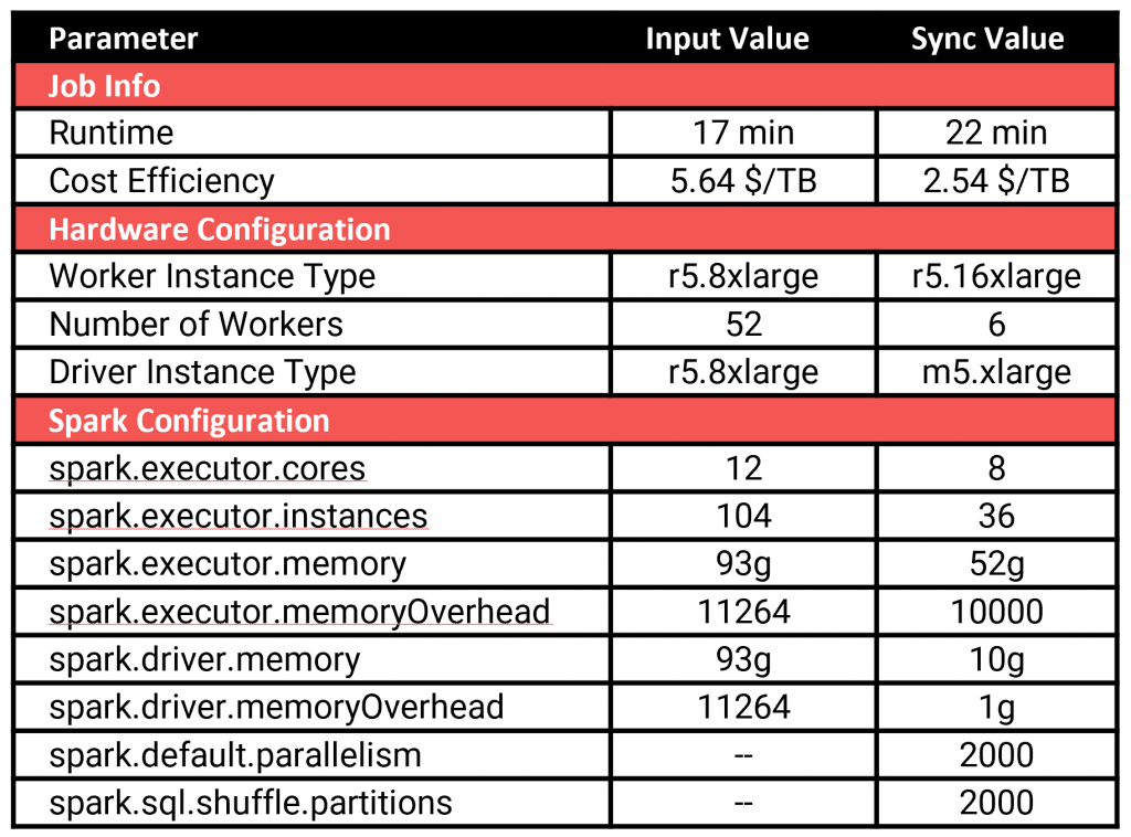
This flexibility of choice is a major utility of the Spark Cluster Gradient. The word “optimal” can mean cheapest to one group, or fastest to another, and the Cluster Gradient gives the right configuration according to each user’s desires. Table 2 shows the input and predicted configurations for this job.

Table 2: Hardware and spark configurations before and after using the Cluster Gradient for the ETL-D job.

The Measurement

When Duolingo actually ran this predicted configuration in their production runs, they instantly saw dramatic cost savings — which was precisely their goal.

The greatest cost savings come from the reduction in cluster size (from 1,664 to 384 vcpu’s). Although the cluster size was reduced by 4x, the runtime only increased slightly from 17 min to 22 min, and cost was reduced by 55%.

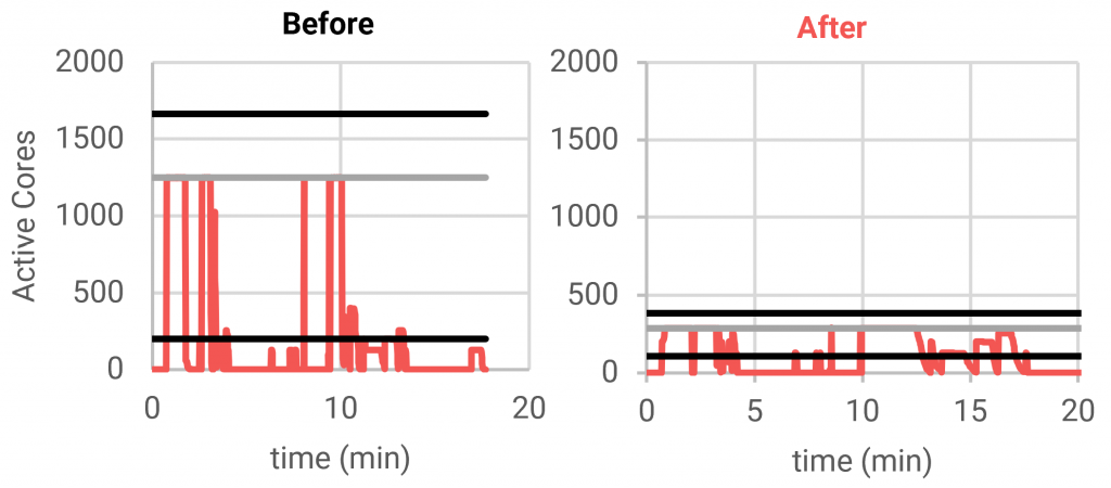
These results can be understood by looking at the activity charts in Figure 5. In the input log, the average number of active cores was only about 1/6th of the cores available to Spark. This indicates that the majority of the job is not well distributed, and most of the cluster time was spent doing nothing. The optimized result reduced the cluster size, bringing the mean activity closer to the available capacity, making the job more efficient and therefore less expensive. Of course, those stages which were well distributed now take longer, resulting in a slightly longer runtime.

Figure 5: Cluster activity for the ETL-D job before and after running Sync’s Spark Cluster Gradient

At first glance it appears that reducing the cluster size more would improve the utilization even further, resulting in even lower costs. However, this is untrue in this case, because increasing the runtime also increases the driver costs and the EBS costs. The Cluster Gradient takes all of these factors into account to estimate the total cost of running a job at various cluster sizes.

The next most impactful change to the job is the driver size, as an on-demand instance for the driver can cost as much as several equivalent spot instances. After analyzing the input log, the Cluster Gradient determined that an m5.xlarge had sufficient memory to handle this job, reducing driver cost by nearly 10x. Lastly, the changes to the Spark configurations are largely to conform to the new hardware configuration, though these settings are necessary for the application to run efficiently on the hardware.

Conclusion – Demo it yourself

This demonstration is just a small example of the complexity built in the Spark Cluster Gradient. Changes to the hardware and Spark settings can impact the runtime of a job in many and often subtle ways. Appropriately accounting for these effects to accurately predict runtime requires the deep mathematical modeling and optimization of the Cluster Gradient, which goes far beyond the capability of simple rule-of-thumb decisions or local optimization techniques. But don’t take our word for it, try out our first solution in the link below on your real production Spark jobs today – we’d love your feedback.

Sync Computing – Configure complex cloud infrastructure for your data/ML workloads based on cost and time, before you submit your jobs to obtain the best performance and value.

Jeffrey Chou

06 Dec 2021

Jeff is the co-founder and CEO of Sync Computing. He holds a PhD from UC Berkeley and was a post-doc at MIT. His interest is in large compute infrastructure and entrepreneurship.