Case Study

How does the worker size impact costs for Apache Spark on EMR AWS?

Jeffrey Chou
03.01.2023

Here at Sync, we are passionate about optimizing data infrastructure on the cloud, and one common point of confusion we hear from users is what kind of worker instance size is best to use for their job?

Many companies run production data pipelines on Apache Spark in the elastic map reduce (EMR) platform on AWS. As we’ve discussed in previous blog posts, wherever you run Apache Spark, whether it be on Databricks or EMR, the infrastructure you run it on can have a huge impact on the overall cost and performance.

To make matters even more complex, the infrastructure settings can change depending on your business goals. Is there a service level agreement (SLA) time requirement? Do you have a cost target? What about both?

One of the key tuning parameters is which instance size should your workers run on? Should you use a few large nodes? Or perhaps a lot of small nodes? In this blog post, we take a deep dive into some of these questions utilizing the TPC-DS benchmark.

Before starting, we want to be clear that these results are very specific to the TPC-DS workload, while it may be nice to generalize, we fully note that we cannot predict that these trends will hold true for other workloads. We highly recommend people run their own tests to confirm. Alternatively, we built the Gradientr for Apache Spark to help accelerate this process (feel free to check it out yourself!).

With that said, let’s go!

The Experiment

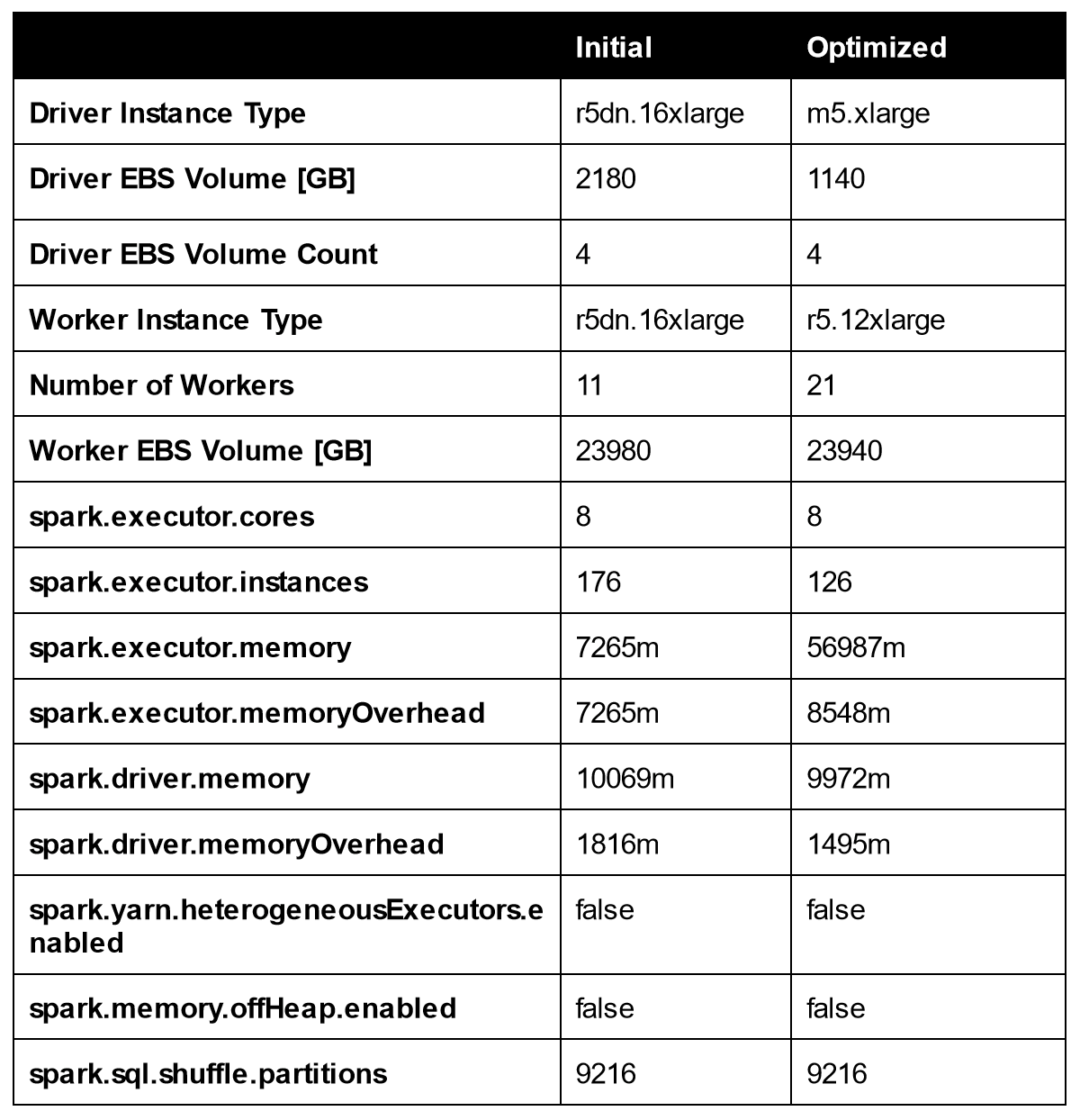
The main question we seek to answer is – “How does the worker size impact cost and performance for Spark EMR jobs?” Below are the fixed parameters we used when conducting this experiment:

EMR Version: 6.2
Driver Node: m5.xlarge
Driver EBS storage: 32 GB
Worker EBS storage: 128 GB
Worker instance family: m5
Worker type: Core nodes only
Workload: TPC-DS 1TB (Queries 1-98 in series)
Cost structure: On-demand, list price (to avoid Spot node variability)
Cost data: Extracted from the AWS cost and usage reports, includes both the EC2 fees and the EMR management fees

Fixed Spark settings:

Spark.executor.cores: 4
Number of executors: set to 100% cluster utilization based on the cluster size
Spark.executor.memory: automatically set based on number of cores

The fixed Spark settings we selected were meant to mimic safe “default” settings that an average Spark user may select at first. To explain those parameters a bit more, since we are changing the worker instance size in this study, we decided to keep the number of cores per executor to be constant at 4. The other parameters such as number of executors and executor memory are automatically calculated to utilize the machines to 100%.

For example, if a machine (worker) has 16 cores, we would create 4 executors per machine (worker). If the worker has 32 cores, we would create 8 executors.

The variables we are sweeping are outlined below:

Worker instance type: m5.xlarge, m5.2xlarge, m5.4xlarge
Number of workers: 1-50 nodes

Results

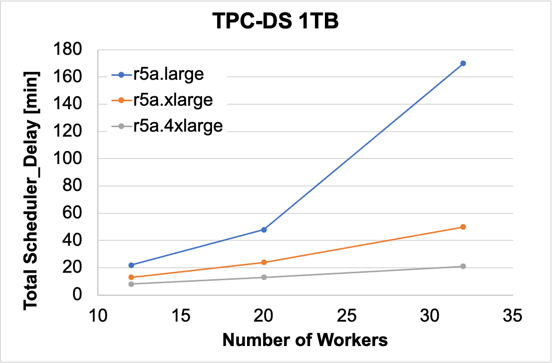
The figure below shows the Spark runtime versus the number and type of workers. The trend here is pretty clear, in that larger clusters are in fact faster. The 4xlarge size outperformed all other cluster sizes. If speed is your goal, selecting larger workers could help. If one were to pick a best instance based on the graph below, one may draw the conclusion that:

It looks like the 4xlarge is the fastest choice

The figure below shows the true total cost versus the number and type of workers. On the cost metric, the story almost flips compared to the runtime graph above. The smallest instance usually outperformed larger instances when it came to lowering costs. For 20 or more workers, the xlarge instances were cheaper than the other two choices.

If one were to quickly look at the plot below, and look for the “lowest points” which correspond to lowest cost, one could draw a conclusion that:

It looks like the 2xlarge and xlarge instance are the lowest cost, depending on the number of workers

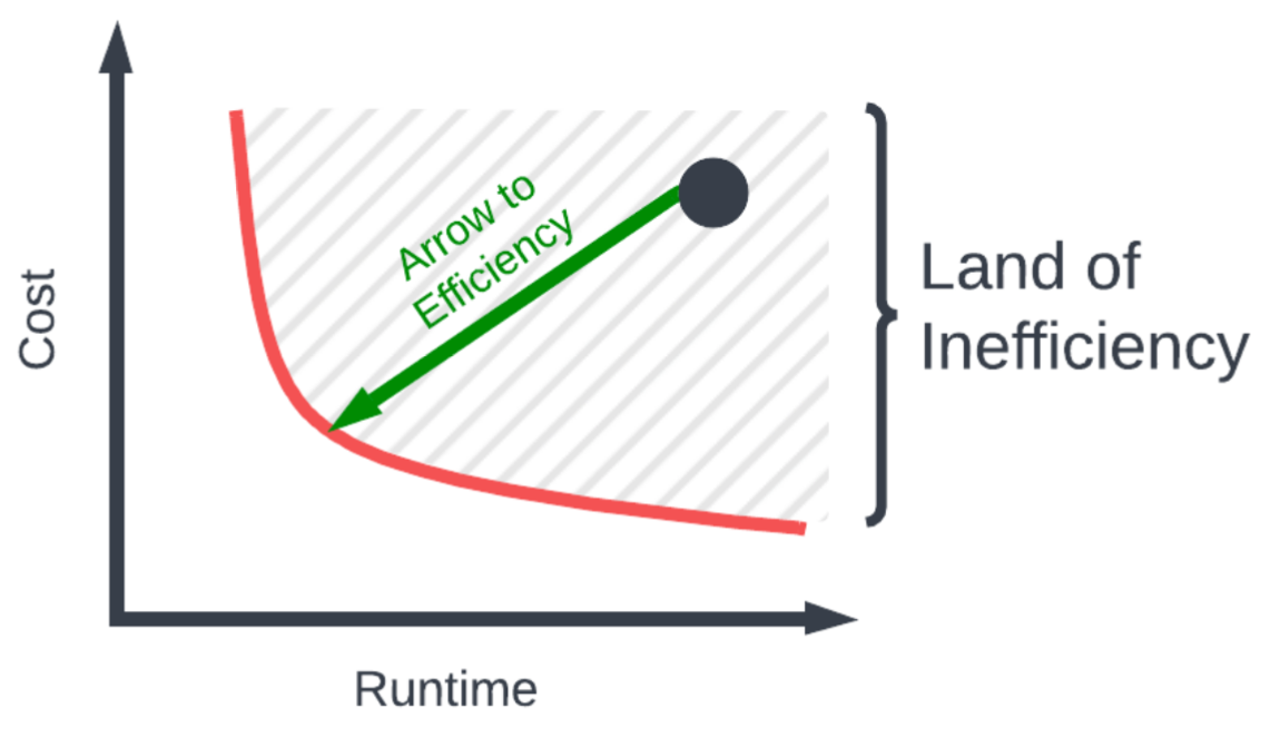
However, the real story comes when we merge those two plots together and simultaneously look at cost vs. runtime. In this plot, it is more desirable to be toward the bottom left, this means the run is both lower cost and faster. As the plot below shows, if one were to look at the lowest points, the conclusion to be drawn is:

It looks like 4xlarge instances are the lowest cost choice… what?

What’s going on here, is that for a given runtime, there is always a lower cost configuration with the 4xlarge instances. When you put it into that perspective, there is little to reason to use xlarge sizes as going to larger machines can get you something both faster and cheaper.

The only caveat here is there is a floor to how cheap and slow the 4xlarge cluster can give you, and that’s with a worker count of 1. Meaning, you could get a cheaper cluster with a smaller 2xlarge cluster, but the runtime becomes quite long and may be unacceptable for real-world applications.

Here’s a generally summary of how the “best worker” choice can change depending on your cost and runtime goals:

Runtime Goal	Cost Goal	Best Worker
<20,000 seconds	Minimize	4xlarge
<30,000 seconds	Minimize	2xlarge
<A very long time	Minimize	xlarge

A note on extracting EMR costs

Extracting the actual true costs for individual EMR jobs from the AWS billing information is not straight forward. We had to write custom scripts to scan the low level cost and usage reports, looking for specific EMR cluster tags. The exact mechanism for retrieving these costs will probably vary company to company, as different security permissions may alter the mechanics of how these costs can be extracted

If you work at a company and EMR costs are a high priority and you’d like help extracting your true EMR job level costs, feel free to reach out to us here at Sync, we’d be happy to work together.

Conclusion

The main takeaways here are the following points:

It Depends: Selecting the “best” worker is highly dependent on both your cost and runtime goals. It’s not straightforward what the best choice is.
It really depends: Even with cost and runtime goals set, the “best” worker will also depend on the code, the data size, the data skew, Spot instance pricing, availability to just name a few.
Where even are the costs? Extracting the actual cost per workload is not easy in AWS, and is actually quite painful to capture both the EC2 and EMR management fees.

Of course here at Sync, we’re working on making this problem go away. This is why we built the Spark Gradient product to help users quickly understand their infrastructure choices given business needs.

Feel free to check out the Gradient yourself here!

You can also read our other blog posts here which go into other fundamental Spark infrastructure optimization questions.

Databricks driver sizing impact on cost and performance

Jeffrey Chou
02.07.2023

As many previous blog posts have reported, tuning and optimizing the cluster configurations of Apache Spark is a notoriously difficult problem. Especially when a data engineer needs to lower costs or accelerate runtimes on platforms such as EMR or Databricks on AWS, tuning these parameters becomes a high priority.

Here at Sync, we will experimentally explore the impact of driver sizing in the Databricks platform on the TPC-DS 1TB benchmark, to see if we can obtain an understanding of the relationship between the driver instance size and cost/runtime of the job.

Driver node review

For those who may be less familiar with the driver node details in Apache Spark, there are many excellent previous blog posts as well as the official documentation on this topic and I will recommend users to read those if they are not familiar. As a quick summary, the driver is an important part of the Apache Spark system and effectively acts as the “brain” of the entire operation.

The driver program runs the main() function, creates the spark context, and schedules tasks onto the worker nodes. Aside from these high level functions, we’d like to note that the driver node is also used in the execution of some functions, most famously when using the collect operation and broadcast joins. During those functions, data is moved to the driver node and if it’s not appropriately sized, can cause a driver side out of memory error which can shut down the entire cluster.

As a quick side note, for broadcast joins, It looks like a ticket has been filed to change this behavior (at least for broadcast joins) in the open source Spark core. So people should be aware that this may change in the future.

How Does Driver Sizing Impact Performance As a Function of the Number Of Workers?

The main experimental question we want to ask is “how does driver sizing impact performance as a function of the number of workers?” The reason why we want to correlate driver size with the number of workers is that the number of workers is a very important parameter when tuning systems for either cost or runtime goals. Observing how the driver impacts the worker scaling of the job is a key part of understanding and optimizing a cluster.

Fundamentally, the maximum number of tasks that can be executed in parallel is determined by the number of workers and executors. Since the driver node is responsible for scheduling these tasks, we wanted to see if the number of workers changes the hardware requirements of the driver. For example, does scheduling 1 million tasks require a different driver instance type than scheduling 10 tasks?

Experimental Setup

The technical parameters of the experiment are below:

Data Platform: Databricks
Compute type: Jobs (ephemeral cluster, 1 job per cluster)
Photon Enabled: No
Fixed parameters:: All worker nodes are i3.xlarge, all configs default
Sweep parameters: Driver instance size (r5a.large, r5a.xlarge, r5a.4xlarge), number of workers
AWS market: On-demand (to eliminate spot fluctuations)
Workload: Databrick’s own benchmark on TPC-DS 1TB (all queries run sequentially)

For reference, here are the hardware specifications of the 3 different drivers used on AWS:

The result

We will break down the results into 3 main plots. The first is below where we look at runtime vs. number of workers for the 3 different driver types. In the plot below we see that as the number of workers increases the runtime decreases. We note here that the scaling trend is not linear and there is a typical “elbow” scaling that occurs. We published previously the general concept of scaling jobs. We observe here that the largest driver, r5a.4xlarge, yielded the fastest performance across all worker sizes.

In the plot below we see the cost (DBU’s in $) vs. number of workers. For the most part we see that the medium sized driver, r5a.xlarge is the most economical, except for the smallest number of workers where the smallest driver size r5a.large was the cheapest.

Putting both plots together, we can see the general summary when we plot cost vs. runtime. The small numbers next to each point show the number of workers. In general, the ideal points should be toward the bottom left, as that indicates a configuration that is both faster and cheaper. Points that are higher up or to the right are more expensive and slower.

Some companies are only concerned about service level agreement (SLA) timelines, and do not actually need the “fastest” possible runtime. A more useful way to think about the plot below is to ask the question “what is the maximum time you want to spend running this job?” Once that number is known, you can then select the configuration with the cheapest cost that matches your SLA.

For example, consider the SLA scenarios below:

1) SLA of 2500s – If you need your job to be completed in 2,500s or less, then you should select the r5a.4xlarge driver with a worker size of 50.

2) SLA of 4000s – If you need your job to be completed in 4,000s or less, then you should select the r5a.xlarge driver with a worker size of 20.

3) SLA of 10,000s – If you need your job to be completed in 10,000s or less, then you should select the r5a.large driver with a worker size of 5.

Key Insights

It’s very convenient to see the scaling trend of all 3 drivers plotted in this manner, as there are several key insights gained here:

There is a general “good” optimal driver for TPC-DS 1TB – across the spectrum, it’s clear that r5a.xlarge is a good choice generally as it is usually cheaper and faster than the other driver sizes. This shows the danger that if your driver is too big or too small, you could be wasting money and time.
At the extremes, driver size matters for TPC-DS 1TB – At the wings of either large clusters (50 workers) or small clusters (5 workers) we can see that the best driver selection can swing between all 3 drivers.
Drivers can be too big – At 12 workers, the r5a.4xlarge performance is slightly faster but significantly more expensive than the other two driver types. Unless that slight speedup is important, it’s clear to see that if a driver is too large, then the extra cost of the larger driver is not worth the slight speedup. It’s like buying a Ferrari to just sit in traffic – definitely not worth it (although you will look cool).
Small driver bottleneck – For the small driver curve (r5a.large), we see that the blue line’s elbow occurs at a higher runtime than the middle driver (r5a.xlarge). This implies that the smaller driver is creating a runtime bottleneck for the entire workload as the cluster becomes larger. The next section will dive into why.

Root cause analysis for the “small driver bottleneck”

To investigate the cause of the small driver bottleneck, we looked into the Spark eventlogs to see what values changed as we scaled the number of workers. In the Spark UI in Databricks, the typical high level metrics for each task are shown below and plotted graphically. The image below shows an example of a single task broken down into the 7 main metrics:

When we aggregated all of these values across all tasks, across all the different drivers and workers, the numbers were all pretty consistent, except for one number: “Scheduler Delay”. For those who may not be familiar, the formal definition from the Databricks Spark UI, is shown in the image below:

“Scheduler delay includes time to ship the task from the scheduler to the executor, and time to send the task result from the executor to the scheduler. If scheduler delay is large, consider decreasing the size of tasks or decreasing the size of task results.”

In the graph below, we plot the total aggregated scheduler delays of all tasks for each of the job configurations vs the number of workers. It is expected that the aggregated scheduler delay should increase for a larger number of workers since there are more tasks. For example, if there are 100 tasks, each with 1s of scheduler delay, the total aggregated scheduler day is 100s (even if all 100 tasks executed in parallel and the “wall clock” scheduler delay is only 1s). Therefore, if there are 1000 tasks, the total aggregated scheduler should increase as well.

Theoretically this should scale roughly linearly with the number of workers for a “healthy” system. For the “middle” and “large” sized drivers (r5a.xlarge and r5a.4xlarge respectively), we see the expected growth of the scheduler delay. However, for the “small” r5a.large driver, we see a very non-linear growth of the total aggregated scheduler delay, which contributes to the overall longer job runtime. This appears to be a large contributor to the “small driver bottleneck” issue.

To understand a bit deeper as to what is the formal definition of Scheduler Delay, let’s look at the Spark source code inside the function AppStatusUtils.scala. At a high level, scheduler delay is a simple calculation as shown in the code below:

schedulerDelay = duration – runTime – deserializeTime – serlializeTime – gettingResultTime

To put it in normal text, scheduler delay is basically a catch-all term, that is the time the task is spent doing something that is not executing, serializing data, or getting results. A further question would be to see which one of these terms is increasing or decreasing due to the smaller driver? Maybe duration is increasing, or maybe gettingResultTime is decreasing?

If we look at the apples to apples case of 32 workers for the “medium” r5a.xlarge driver and the “small” r5a.large driver, the runtime of the “small” driver was significantly longer. One could hypothesize that the average duration per task is longer (vs. one of the other terms becoming smaller).

In summary, our hypothesis here is that by reducing the driver size (number of VCPUs and memory), we are incurring an additional time “tax” on each task by taking, on average, slightly longer to ship a task from the scheduler on the driver to each executor.

A simple analogy here is, imagine you’re sitting in bumper to bumper traffic on a highway, and then all of a sudden every car (a task in Spark) just grew 20% longer, if there are enough cars you could be set back miles.

Conclusion

Based on the data described above, the answer to the question above is that inappropriately sized drivers can lead to excess cost and performance as workers scale up and down. We present a hypothesis that a driver that is “too small” with too few VCPUs and memory, could cause, on average, an increase in the task duration via an additional overhead in the scheduler delay.

This final conclusion is not terribly new to those familiar with Spark, but we hope seeing actual data can help create a quantitative understanding on the impact of driver sizing. There are of course many other things that could cause a poor driver to elongate or even crash a job, (as described earlier via the OOM errors). This analysis was just a deep dive into one observation.

I’d like to put a large caveat here that this analysis was specific to the TPC-DS workload, and it would be difficult to generalize these findings across all workloads. Although the TPC-DS benchmark is a collection of very common SQL queries, in reality individual code, or things like user defined functions, could throw these conclusions out the window. The only way to know for sure about your workloads is to run some driver sizing experiments.

As we’ve mentioned many times before, distributed computing is complicated, and optimizing your cluster for your job needs to be done on an individual basis. Which is why we built the Apache Spark Autotuner for EMR and Databricks on AWS to help data engineers quickly find the answers they are looking for.

Is Databricks autoscaling cost efficient?

Jeffrey Chou
01.20.2023

Here at Sync we are always trying to learn and optimize complex cloud infrastructure, with the goal to help more knowledge to the community. In our previous blog post we outlined a few high level strategies companies employ to squeeze out more efficiency in their cloud data platforms. One very popular response from mid-sized to large enterprise companies we hear a lot of is:

“We use Autoscaling to minimize costs”

We wanted to zoom into this statement to really understand how true it is, and to get a better understanding of the fundamental question

“Is autoscaling Apache Spark cost efficient?”

To explain in more detail, we wanted to investigate the technical side of Autoscaling and really dive deep into a specific example. Because of this we chose to begin with a gold standard workload to analyze, the TPC-DS benchmark, just to minimize any argument being made that we cherry picked a weird workload to skew the final answer. Our goal here is to be as technical and informative as possible about a few workloads – we are not trying to perform a broad comprehensive study (that would take a long time). So let’s begin:

What is Autoscaling?

For those who may not know, Autoscaling is the general concept that a cluster should automatically tune the number of workers (or instances on AWS) based on the needs of your job. The basic message told to companies is, autoscaling will optimize the cluster for your workload and minimize costs.

Technically, Autoscaling is usually a reactive algorithm that measures some utilization metric inside your cluster to determine if more or less resources are needed. While this makes logical sense, in reality the complexity of Apache Spark and constantly changing cloud infrastructure make this problem highly unpredictable.

In the Databricks UI, autoscaling is just a simple checkbox that many people may overlook. The choice people make by selecting that box could impact their overall performance significantly.

Since many people use Databricks or EMR, the exact algorithm they employ is behind closed doors, so we don’t know the exact details of their logic. The only thing we can do is measure their performance.

Experiment Setup

Our goal is to provide a technical study of Autoscaling from a novice’s point of view. Meaning, our base case to compare against will be whatever “default” settings Databricks suggests. We are not comparing against the global best or against an expert who has spent many days optimizing a particular cluster (who we think would probably do an awesome job).

Data Platform: Databricks
Compute type: Jobs (ephemeral cluster, 1 job per cluster)
Photon Enabled: No
Baseline configuration: Default params given to users at spin up
AWS market: Driver on-demand, workers on spot with 100% on-demand fall back
Workload: Databrick’s own benchmark on TPC-DS 100GB (all 99 queries run sequentially)

To keep things simple, we ran 3 comparison job runs:

Fixed 8 Nodes – a fixed 8 node cluster using the default machine types suggested to us in the Databricks UI.
Fixed 2 Nodes w/ Gradient- We use our Apache Spark Gradient product to recommend an optimized fixed custer to give us the lowest cost option (runtime not optimized). The recommendation was to use 2 nodes (with different instance types than default)
Autoscaler 2-8 Nodes – We used the default UI settings in Databricks here.

	Fixed Cluster	Fixed Cluster (Gradient)	Autoscaler 2-8 Nodes
No. of Workers	8	2	2-8
Driver Node	i3.xlarge	r5a.large	i3.xlarge
Worker Nodes	i3.xlarge	i3.2xlarge	i3.xlarge
Runtime [s]	1593	2441	2834
DBU Cost [$]	0.6	0.39	0.73
AWS Cost [$]	0.92	0.92	1.35
Total Cost [$]	1.52	1.31	2.08

The results

To our surprise, of the 3 jobs run, the default autoscaler performed the worst in both runtime and cost. Both a fixed cluster of 8 nodes and 2 nodes, outperformed autoscaling in both time and cost. The Sync optimized cluster outperformed autoscaling by 37% in terms of cost and 14% in runtime.

To examine why the autoscaled cluster performed poorly, let’s look at the number of workers created and shut-down over time, in comparison to the fixed 2 node cluster. The figure below tells the basic story, that the autoscaled cluster spent a lot of time scaling up and down, tuning itself to the workload itself. At first glance, that is exactly what autoscaling is supposed to do, so why did the autoscaled cost and runtime perform so poorly?

The main reason, from what we can tell, is that there is a time penalty for changing the cluster size – specifically in upsizing the cluster. We can see from the cluster event log below, that the time between “RESIZING” and “UPSIZE_COMPLETED” can span several minutes. Based on the Spark UI, the executors don’t get launched until “UPSIZE_COMPLETED” occurs, so no new computing occurs until this step is achieved.

Another observation here is that in order for us to run the TPC-DS benchmark, we had to run an init_script to install some code at the start of the job. Based on the cluster event log below, it looks like every time it upsizes new machines, they have to reinstall all the init_scripts each time which costs time and money. This is something to consider, where if your job requires you to load specific init_scripts, this would certainly negatively impact the autoscaling performance.

So to summarize, you are paying for the “ramp up time” of new workers during autoscaling, where no computing is occurring. The more often your cluster upsizes, the more you will be waiting and paying.

Databricks mentions that using pools can help speed up autoscaling, by creating a pool of “warm” instances ready to be kicked off. Although you are not charged DBU’s, you do still have to pay AWS’s fees for those machines. So in the end, it still depends on your workload, size of cluster, and use case if the pools solution makes sense.

Another issue is the question of optimizing for throughput. If 3 nodes processes the data at the same rate as 8 nodes, then ideally autoscaling should stop at 3 nodes. But it doesn’t seem like that’s the case here, as auto-scaling just went up to the max workers set by the user.

The optimized fixed cluster looks at cost and throughput to find the best cluster, which is another reason why it is able to outperform the autoscaling solution.

Some follow up questions:

Is this just a TPC-DS specific artifact?

We ran the same tests with two other internal Spark jobs, which we call Airline Delay and Gen Data, and observed the same trend – that the Autoscale cluster was more expensive than fixed clusters. The amount of Autoscaling fluctuation was much less for Airline delay, so we noticed the advantage of a fixed cluster was reduced. Gen Data is a very I/O intense job, and the autoscaler actually did not scale up the cluster beyond 2 nodes. For the sake of brevity, we won’t show those details here (feel free to reach out if there are more questions).

We just wanted to confirm that these results weren’t specific to TPC-DS, and if we had more time we could do a large scale test with a diverse set of workloads. Here we observed the optimized fixed cluster (using the Sync Apache Spark Gradient) achieved a 28% and 65% cost savings over default autoscaling for Airline Delay and Gen Data respectively.

What if we just set Autoscaling to 1-2 nodes (instead of 2-8)?

We thought that if we just changed the autoscaling min and max to be near what the “Fixed 2 node gradient” cluster was, then it should get about the same runtime and cost. To our surprise, what happened was the autoscaler bounced back and forth between 1 and 2 nodes, which caused a longer job run than the fixed cluster. You can see in the plot below, we added the autoscaling job from 1-2 nodes on the worker plot. Overall the cost of the fixed 2 nodes cluster was still 12% cheaper than the autoscaled version of the same cluster with 1-2 nodes.

What this results indicates is that the parameters of min/max workers in the autoscaler are also parameters to optimize for cost and require experimentation.

How does the cost and runtime of the job change vs. varying the autoscaling max worker count?

If the cost and runtime of your job changes based on the input into max and min worker count, then autoscaling actually becomes a new tuning parameter.

The data below shows what happens if we keep the min_worker = 2, but sweep the max_worker from 3 to 8 workers. Clearly both cost and runtime vary quite a bit compared to the Max Worker count. And the profiles of these slopes depends on the workload. The bumpiness of the total cost can be attributed to the fluctuating spot prices.

The black dashed line shows the runtime and cost performance of the optimize fixed 2 node cluster. We note that a fixed cluster was able to outperform the best optimal autoscaling configuration for cost and runtime for the TPC-DS workload.

How did we get the cost of the jobs?

It turns out obtaining the actual cost charged for your jobs is pretty tedious and time consuming. As a quick summary, below are the steps we took to obtain the actual observed costs of each job:

Obtain the Databricks ClusterId of each completed job. (this can be found in the cluster details of the completed job under “Automatically added tags”)
In the Databricks console, go to the “manage account>usage tab”, filter results by tags, and search for the specific charge for each ClusterId. (one note: the cost data is only updated every couple of hours, so you can’t retrieve this information right after your run completes)
In AWS, go to your cost explorer, filter by tags, and type in the same cluster-id to obtain the AWS costs for that job (this tag is automatically transferred to your AWS account). (Another note, AWS updates this cost data once a day, so you’ll have to wait)
Add together your DBU and AWS EC2 costs to obtain your total job cost.

So to obtain the actual observed total cost (DBU and AWS), you have to wait around 24 hours for all of the cost data to hit their final end points. We were disappointed to see we couldn’t see the actual cost in real time.

Conclusion

In our analysis, we saw that a fixed cluster could outperform an autoscaled cluster in both runtime and costs for the 3 workloads that we looked at by 37%, 28%, and 65%. Our experiments showed that by just sticking to a fixed cluster, we eliminated all of the overhead that came with autoscaling which resulted in faster runtimes and lower costs. So ultimately, the net cost efficiency all depends on if the scaling benefits outweigh the negative overhead costs.

To be fair to the autoscaling algorithm, it’s very difficult to build a universal algorithm that reactively works for all workloads. One has to analyze the specifics of each job in order to truly optimize the cluster underneath and then still experiment to really know what’s best. This point is also not specific to Databricks, as many data platforms (EMR, Snowflake, etc) also have autoscaling policies that may work similarly.

To summarize our findings, here are a few high level takeaways:

Autoscaling is not one size fits all – Cluster configurations is an extremely complicated topic that is highly dependent on the details of your workload. A reactive autoscaling algorithm and the overheads associated with changing the cluster is a good attempt, but does not solve the problem of cluster optimization.
Autoscaling still requires tuning – Since Autoscaling is not a “set and forget” solution, it still requires tuning and experimentation to see what min and max worker settings are optimal for your application. Unfortunately, since the autoscaling algorithm is opaque to users, the fastest way to determine the best settings is to manually experiment.
So when is autoscaling good to use for batch jobs? It’s difficult to provide a general answer because, like mentioned above, it’s all dependent on your workload. But perhaps two scenarios I could see are (1) if your job has long periods of idle time, then autoscaling should shut down the nodes correctly, or (2) you are running ad-hoc data science experiments and you are prioritizing productivity over costs. Scenarios (1) and (2) could be the same thing!
So what should people do? If cost efficiency of your production level Databricks jobs is a priority, I would heavily consider performing an experiment where you select a few jobs, switch them to fixed clusters, and then extract the costs to do a before and after analysis – just like we did here.

The challenge of the last bullet is, what is the optimal fixed cluster? This is an age-old question that required a lot of manual experimentation to determine in the past, which is why we built the Apache Spark Gradient to figure that out quickly. In this study, that is how I found the optimal fixed clusters with a single file upload, without having to run numerous experiments.

Maybe autoscaling is great for your workloads, maybe it isn’t, unfortunately the answer is really “it depends.” There’s only one way to really find out – you need to experiment.

Top 3 trends we’ve learned about the scaling of Apache Spark (EMR and Databricks)

Jeffrey Chou
08.02.2022

We launched the Gradient for Apache Spark several months ago, and have worked with many companies on analyzing and optimizing their Apache Spark workloads for EMR and Databricks. In this article, we summarize cluster scaling trends we’ve seen with customers, as well as the theory behind it. The truth is, cluster sizing and configuring is a very complex topic and is different for each workload. Some cloud providers ignore all of the complexities and offer simple “T-Shirt” sizes (e.g. small, large, xlarge), while although great for quick testing of jobs, will lead to massive cost inefficiencies in production environments.

The Sync Gradient for Apache Spark makes it easy to understand the complex tradeoffs of clusters, and enables data engineers to make the best cloud infrastructure decisions for their production environments.

Try for free: Gradient for Apache Spark

The Theory

In any distributed computing system (even beyond Apache Spark), there exist well known scaling trends (runtime vs. number of nodes), as illustrated in the images below. These trends are universal and fundamental to computer science, so even if you’re running Tensorflow, OpenFOAM (computational fluid dynamics solver), or MonteCarlo simulations on many nodes, they will all follow one of the three scaling trends below:

Standard Scaling: As more and more nodes are added, the runtime of the job decreases, but the cost also increases. The reason is because adding more nodes is not free computationally, there are usually additional overheads to runtime such as being network bound (e.g. shuffles in Spark), compute bound, I/O bound, or memory bound. As an example, doubling the number of nodes to run your job results in a runtime of more than half of the original runtime if they exhibit standard scaling.

At some point, adding more nodes has diminishing returns and the job stops running faster, but obviously cloud costs start rising (since more nodes are being added). We can see point B here is running on let’s say, 5 nodes, but point A is running on 25 nodes. Running your job at point A is significantly less cost efficient and you may be wasting your money.

Embarrassingly Parallel: This is the case when adding more nodes actually does linearly decrease your runtime, and as a result we see a “flat” cost curve. This is traditionally known in the industry as “embarrassingly parallel” because there are no penalties for adding more nodes. This is usually because there is very little communication between nodes (e.g. no shuffles in Spark), and each node just acts independently.

For example at point B we are running at 5 nodes, but point A we’re running at 25 nodes. Turns out, although your number of nodes from A to B went up by 5x, your runtime also went down by 5x. So they both cancel out and you basically have a flat cost curve. In this case, you are free to increase your cluster size, and decrease your runtime for no extra cost! Due to the computational overheads mentioned above though, this case is quite rare and will eventually stop at large enough nodes (when exactly depends on your code).

Negative Scaling: This is the interesting case when running with more nodes is both cheaper and faster (the complete opposite of “Standard Scaling”). The reason here is that some overheads could actually decrease with larger cluster sizes. For example, there could be a network or disk I/O bound issue (e.g. fetch time waiting for data), where having more nodes increases the effective network or I/O bandwidth and makes your jobs run a lot faster. If you have too few nodes, then network or I/O will be your bottleneck as your Spark application gets hung up on fetching data. Memory bound jobs could also exhibit this behavior if the cluster is too small and doesn’t have enough memory, and there exists significant memory overhead.

For example at point B, we are running at 5 nodes, but now we only have 5 machines performing data read/write. But at point A we have 25 nodes, we have 5x more bandwidth on read/write, and thus the job runs much faster.

Real Customer Plots

The 3 scaling trends are universal behaviors of any distributed compute system, Apache Spark applications included. These scaling curves exist whether you’re running open source Spark, EMR, or Databricks — this is fundamental computer science stuff here.

When we actually started processing customer logs, we noticed that the jobs weren’t even on the proper scaling curve, due to the improper configurations of Spark. As a result, we saw that customers were actually located in the “Land of Inefficiency” (as shown by the striped region below), in which they were observing both larger costs and runtime, for no good reason.

For example if you set your workers and memory settings improperly, the result you’d see in the gradient is a black “current” dot in the “Land of Inefficiency.” The entire goal of the gradient is to provide an easy and automatic way for customers to achieve an efficient Spark cluster.

Standard Scaling — In the 3 screen shots below, we see the classic standard scaling for customer jobs. We see the classic “elbow” curve as described above. We can see that here in all 3 cases, all of the users were in the “Land of Inefficiency.” Some of the runtime and cost savings went up to 90%, which was amazing to see. Users can also tune the cost/runtime, based on their company’s goals.

Embarrassingly Parallel: In the screen shots below, we see almost flat curves for these jobs. In these cases the jobs were almost entirely CPU bound, meaning there was little communication between nodes. As a result, adding more nodes linearly increased the runtime. In this case, the jobs were still in the “Land of Inefficiency”, so substantial cost/runtime savings could still be achieved.

Negative Scaling — In the screen shots below, we see the negative scaling behavior. The issue here is a large amount of fetch wait time (e.g. network I/O) that causes larger clusters to be substantially more efficient than smaller clusters. As a result, going to larger clusters will be more advantageous for both cost and runtime.

Conclusion

We hope this was a useful blog for data engineers. As readers hopefully see, the scaling of your big data jobs is not straightforward, and is highly dependent on the particularities of your job. The big question is always, what is the bottleneck of your job? Is it CPU, network, disk I/O, or memory bound? Or perhaps it is a combination of a few things. The truth is, “it depends” and requires workload specific optimization. The Gradient for Apache Spark is an easy way to understand your workload, bring you out of the “Land of Inefficiency”, and optimize your job depending on the type of scaling behavior it exhibits.

One question we get a lot is — what about multi-tenant situations when one cluster is running hundreds or thousands of jobs? How does the Gradient take into account other simultaneous jobs? This solutions requires another level of optimization, and one we recently published a paper on entitled “Global Optimization of Data Pipelines on the Cloud”

References

Optimize Databricks Clusters Based on Cost and Performance

Jeffrey Chou
04.10.2022

Databricks is increasingly one of the most popular platforms to run Apache Spark, as it provides a relatively friendly interface that allows data scientists to focus on the development of the analytical workloads—and efficiently build extract load transform (ELT) type operations. The multiple options it provides, by virtue of being built on top of Apache Spark, like supported languages (Java, Python, Scala, R, and SQL) and rich libraries (MLlib, graphX, sparknlp ) makes it a very attractive choice for a data compute platform.

That said, without careful consideration when creating clusters to run big data workloads, costs and runtime can easily expand beyond initial assumptions. And despite its importance, adjusting proper compute parameters is both time intensive and not immediately clear to new users.

Configuring compute infrastructure for Databricks to hit cost/performance goals can be daunting. We have been approached by many mid-sized B2B data service providers who have had the desire to improve their Databricks usage. Since their customer’s product is data, their Databricks bill and engineering time directly impacts their profit margin.

After careful investigation, we have been able to provide guidance on several workloads. Read below to see our explanation into Databricks parameters, and our case study showing how we reduced Databricks cost by increasing cluster efficiency and runtime.

First off, what are clusters in Databricks?

Databricks defines clusters as ”a set of computation resources and configurations on which you run data engineering, data science, and data analytics workloads.” In plain English this means a Databricks cluster is a combination of hardware and virtual instructions that can execute your Databricks code, referred to as your “workload”, within your Databricks workspace. They are the backbone of you get things done.

A cluster to run Databricks jobs is composed of a single driver node and possibly multiple worker nodes. Nodes themselves have hardware sucb as a CPU, memory, DISKs and cashe, used to host Spark and manage clusters. Databricks clusters can come in many forms such as notebooks (which are a set of commands) automated jobs, delta-live tables, and SQL queries. These cluster types often come in different pricing tiers.

Specific instance types must be selected for each driver or group of workers, of which there are hundreds of possible options. Selecting which cluster type to use, the pricing, cluster policies, autoscaling, and even which Databricks runtime can be a daunting task when running standard ETL pipelines.

In order to run any of those workloads, a user must first create clusters from their cloud provider, such as AWS, Microsoft Azure Databricks, or Google Cloud. Which type of cluster you create depends on everything from your data lake and Databricks runtime version to your individual workflow.

Below we go through cluster types and cluster modes and how to understand and select the type appropriate for your needs.

The Importance of Cluster Modes and Clusters Types In Databricks

When referencing clusters in Databricks, you’ll hear reference to both cluster type and cluster mode. It’s important to understand the difference to get high performance in your jobs.

There are two many cluster types: interactive (or all-purpose cluster) and job cluster.

Interactive clusters allow you to analyze data collaboratively with interactive notebooks, and can be created using the Databricks UI via notebooks.
Job clusters on the other hand are designed to fun fast automated workloads, such as ones using an API. Job clusters are created whenever you create a new job via CLI or Rest API. For this reason, interactive clusters can be stopped and restarted while job clusters must terminate once the job ends and cannot be restarted.

Cluster modes on the other hand refer more to the shared usage and permissions of a cluster.

Standard clusters (now called “No Isolation Shared Access Mode”) are the defaults and can be used with Python, R, Scala and SQL. They can be shared by multiple users with no isolation between the users.
High concurrency clusters (now called “Shared Access Mode”) are cloud-managed resources, meaning they share virtual machines across the network to provide maximum resource utilization for each notebook. This is used both for minimum query latency, as well as for users to utilize table access control, which is not supported in standard clusters. Workloads supported in these modes of clusters are in Python, SQL and R.
Lastly, single node clusters have only one node for the driver. As the name implies, this is for a single user and in this mode, the spark job runs on the driver note itself—as there is no worker node available in this job

Standard clusters and single nodes terminate after 120 minutes by default, whereas high concurrency clusters do not. It’s important to note the mode during the cluster creation process as it cannot be changed and you must create a new cluster to update the mode.

How Optimizing Databricks Clusters Can Help Reduce Databricks Costs and Accelerate Runtimes

Properly configuring your databricks clusters can help save money by saving time — Configuring compute infrastructure for Databricks to hit cost/performance goals can be daunting. (Image by author)

To that extent, a mid-sized B2B customer company that provides data services to businesses, approached Sync Computing with the desire to improve their Databricks usage. Since the customer’s product is data, their Databricks bill and engineering time directly impacts their profit margin.

After careful investigation, we were able to provide guidance on several workloads. This particular job, after our collaboration, resulted in 34% cost reduction and 17% runtime reduction. (Though we have achieved greater gains with other Databricks jobs.) This means, we were able to not only reduce their cost but enable better capabilities around meeting their data SLAs (service level agreements).

The chart below depicts their initial cost and runtime and the associated improvements we achieved together. The gray dots represent different predictions with varying numbers of workers of the same instance type.

This image shows how to save 34% on server costs by reducing runtime in Databricks jobs. — Results of the gradient prediction and real run by the customer. (Image by author)

To achieve the result above, a full list of the parameters changed by Gradient is shown in table 1. By switching instance types, number of workers, memory and storage parameters all simultaneously, Gradient performs a global optimization to achieve the desired cost and performance goals selected by the user.

Table 1. Comparison of the original vs optimized Databricks configurations. (Image by author)

Out of the collaboration, several highlights may provide value to other Databricks users. We have detailed them below (in no particular order).

Reduce Costs by Right-sizing Worker Instance Types, number of workers, and Storage

Without much insight about which instance types are worth selecting for specific workloads, it’s tempting to assemble clusters that are composed of large worker nodes with significant attached storage. This strategy is sensible for focusing not on infrastructure during development of data pipelines but once these pipelines are in production, it is worth the effort to look at cluster composition to save costs and runtime. In our collaboration with the customer, we discovered that they had the opportunity to downsize their worker node instance type, number of workers and assign appropriate storage. See figure below that illustrates this point. Our recommendation actually includes smaller worker instances and increased EBS (storage). The initial cluster included 11 r5dn.16xlarge instances and the recommended cluster included a larger number of workers (21) but smaller instance types, r5.12xlarge. The resulting cost decrease is mostly due to smaller instances despite an increase in the number. Balancing instance types and the number of workers is a delicate calculation, if done incorrectly could erase all potential gains. Gradient predicts both values simultaneously for users, to eliminate this tricky step. The costs associated with the worker EC2 instances (shown in salmon) represents where the major cost reduction occurred.

We note that switching instances is not trivial, as it may impact other parameters. For example in this case, the r5dn instance type has attached storage. Moving to the r5 instance type requires adding the appropriate amount of EBS storage hence the small increase in the worker EBS costs. Gradient takes this into account and auto-populates the parameters such as these when suggesting to switch instance types.

The cost impact of right sizing the driver node. (Image by author)

Reduce Costs by Right-sizing Driver Instance Type

Databricks provides a wide range of instance types to choose from when setting the driver and worker nodes. The plethora of options stems from the variety of compute the underlying cloud provider (AWS, Azure and GCP) put forth. The number of options can be overwhelming. A common pattern among Spark users involves choosing the same instance type for both worker and driver nodes. We have been able to help folks, like the customer, tune their cluster settings to choose more tailored driver instance types. By avoiding over-provisioning of driver nodes, the cost contribution of the driver can be reduced. This approach tends to yield strong benefits in scenarios where the driver node uses ON-DEMAND instances and the worker nodes are using SPOT instances. The benefits are more pronounced when the cluster has fewer workers.

The chart below shows the cost breakdown of a four worker node cluster. Initially, the cluster consisted of a ON-DEMAND driver m5.12xlarge instance with four SPOT m5.12xlarge workers instances. By right-sizing the driver node to a m5.xlarge instance, a 21% cost reduction is achieved. The salmon-colored portion represents the cost contribution of the change in driver instance type. The right-sizing must avoid under-provisioning so the appropriate spark configuration parameters need to be adopted. That is what the Gradient enables. A small but noticeable increase in the worker costs is related to a slight increase in the runtime associated with the driver instance change.

The cost impact of rightsizing the worker node. (Image by author)

The impact of Spot Availability on Runtime

Using spot instances for worker nodes is a great way to save on compute costs. the customer adopted this practice prior to our initial conversations. However, the cost-saving strategy may actually result in longer runtimes due to availability issues. For large clusters, Databricks may start the job even with only a fraction of the desired total number of target worker nodes. As a result, the data processing throughput is slowly ramped up over time resulting in longer runtimes compared to the ideal case of having all the desired workers from the start. In addition, it is also possible for worker nodes to drop off, due to low Spot availability, during a run of a job and come back via Databricks Autorecovery feature. As a consequence, the total runtime for the cluster will be longer than for a cluster that has the full target number of workers for the entire job.

The chart below presents how Sync helped the customer accelerate their Databricks jobs by 47% by switching to a higher availability instance. The black line represents the run with up to 18 r5dn.16xlarge workers. The salmon line represents the run with 32 c5.12xlarge workers. The AWS Spot Advisor (see link) indicated that the r5dn.16xlarge instance type typically had a higher frequency of interruption, at times 10%-15% greater, than the c5.12xlarge instance type. As we see below, this small difference in interruption can lead to almost a 2x change in runtime.

The run with the c5.12xlarge workers (“low interruptibility”) had no difficulty in assembling the targeted 32 worker count from the beginning. In contrast, the run with the r5dn.16xlarge workers (“high interruptibility”) took a few minutes to start the job but with only 5 of the targeted 18 workers count. It took over 200 minutes to increase the node count to only 15 nodes, never reaching the fully requested amount of 18. Switching worker instance types also requires updates to the spark parameters (e.g. spark.executor.cores, executor memory, number of executors), fortunately Gradient adjusts these parameters as well for each instance type, making it easy for users. Gradient makes cluster configuration recommendations that take into account availability. Databricks users, like the customer, can take advantage of the cost benefits of spot instances with confidence that unforeseen availability will not negatively impact their job runtimes.

By selecting Spot instances with higher availability, Customer’s runtime accelerated by 47%. (Image by author)

Conclusion

The compute infrastructure on which Databricks runs can have a large impact on the cost and performance of any production job. Because the cloud offers an almost endless array of compute options, understanding how to select which cloud configurations to use can lead to an intractable search space. At Sync our mission is to make this problem go away for data engineers everywhere.

How Duolingo reduced their EMR job cost by 55%

Jeffrey Chou
12.06.2021

Launch to the cloud based on cost and time: This article explains Sync Computing’s Spark Cluster Gradient Solution and how it was used to reduce Duolingo’s AWS EMR Spark costs by up to 55%. This solution eliminates the inefficient manual tuning and guesswork currently used when configuring Spark clusters and settings to provide the best cost, performance, and reliability — without any code changes.

The Problem with Spark Infrastructure

Determining cloud infrastructure settings to optimize job cost and speed for modern Spark jobs is neither practical nor possible for cloud developers. Even with optimal settings for one job, Spark jobs vary daily in code base, data sizes, and cloud spot pricing resulting in wide variations of cost/performance to developers. Most cloud users rely on simple rules of thumb or recommendations from co-workers or past jobs on what settings should be selected. Optimizing these choices requires sweeping through instance types, cloud settings, and spark configurations, a task no busy data engineer has time for.

What if it were possible to explore the effects of hardware changes without having to actually rerun jobs? Buried within the output of every Spark run is a trove of information connecting its performance to the underlying hardware. When combined with deep mathematical modeling, this data can be used to predict application performance on different cloud hardware configurations. This is the core idea behind Sync’s first solution, the Spark Cluster Gradient.

How Sync Spark Cluster Gradient can Help

Sync’s Spark Cluster Gradient removes the burden of choosing the right AWS cluster hardware and spark configurations for your recurring production Spark applications. Using only your most recent Spark eventlog and its associated cluster information, the Cluster Gradient returns the optimal cluster and spark configurations for your next run.

Whether “optimal” to you means the fastest, cheapest, or somewhere in between, the Cluster Gradient will give you the appropriate settings for your needs.

Figure 1: Example configuration selections from the Spark Cluster Gradient. These options are presented to a user within minutes of uploading a Spark eventlog.

How Sync Spark Cluster Gradient works

The Cluster Gradient works by mathematically modeling the task-level details of a spark eventlog and calculating how those details will change on different hardware configurations, resulting in an estimate of the runtime on each set of hardware.

Runtime estimates are combined with the latest AWS pricing and reliability information to yield performance estimates (runtime and cost) for each configuration. An optimization calculation is performed to search through all the configurations to pick the best options for the user.

Figure 2: Basic workflow of the Spark Predictor

Duolingo’s Situation

Duolingo builds the world’s #1 language learning application serving over 40 million monthly active users. As a cloud native company, Duolingo processes terabytes of data daily on the cloud, leading to exorbitant costs. Utilizing the cloud efficiently directly impacts the company’s bottom line.

In the following section, we demonstrate a case study of this solution’s use with Duolingo. The experiment follows the workflow depicted in Figure 2.

Duolingo has a number of recurring production Spark jobs run on AWS EMR, which when run daily or even multiple times per day, incur substantial costs over the course of a year. Their #1 priority was to reduce costs, even at the expense of runtime. Figuring out the best configuration on their own would require extensive manual testing and parameter sweeps, a many-hour task no engineer has the bandwidth for.

Sync presented them with the Spark Cluster Gradient, which would get rid of manual experimenting, to instantly reduce their cloud costs on two of their ETL jobs. Basic information of these jobs is outlined in Table 1.

Job	Input Runtime (min)	Input Data Size (TB)	Input Cost ($)
ETL-D	18	2	6
ETL-P	113	5	101

Table 1

The most recent eventlog from each job was run through the Cluster Gradient and the configurations which yielded the lower cluster costs were used in the subsequent runs. The results of this experiment are depicted in Figure 3. For both jobs, the Sync Optimized configuration resulted in a substantial reduction in cost, without touching any code for an easy and fully reversible demonstration.

Figure 3: Cost efficiency of three Spark jobs before and after using the Sync Spark Cluster Gradient

The Prediction

Figure 4 shows a subset of the predictions using Duolingo’s ETL-D log. Three instance types are shown, where each point on the respective curve represents a different number of workers. Performance estimates of the input, predicted, and measured jobs are indicated by the red, green, and blue triangles, respectively.

Figure 4: Performance predictions on varying hardware configurations for the ETL-D job. The performance points of the input, prediction, and measurement are indicated by the triangles.

In this example, a small number of workers in the prediction results in long-running but inexpensive jobs. As the number of workers increases, the application is expected to be faster but costlier. The initial input configuration was deep in the plateau of diminishing returns of cluster scaling. The recommendation was therefore to reduce the number of workers in order to move away from the runtime plateau.

The key insight enabled by the Cluster Gradient is given by the knowledge of where your current job lies on the performance curve, and what you need to change to get to another point on that curve. In Duolingo’s case, cost was the only relevant parameter. On the other hand, if runtime was a critical parameter, then it would be easy to pick another point on this curve that runs nearly as fast as the original job but still with significant cost savings.

This flexibility of choice is a major utility of the Spark Cluster Gradient. The word “optimal” can mean cheapest to one group, or fastest to another, and the Cluster Gradient gives the right configuration according to each user’s desires. Table 2 shows the input and predicted configurations for this job.

Table 2: Hardware and spark configurations before and after using the Cluster Gradient for the ETL-D job.

The Measurement

When Duolingo actually ran this predicted configuration in their production runs, they instantly saw dramatic cost savings — which was precisely their goal.

The greatest cost savings come from the reduction in cluster size (from 1,664 to 384 vcpu’s). Although the cluster size was reduced by 4x, the runtime only increased slightly from 17 min to 22 min, and cost was reduced by 55%.

These results can be understood by looking at the activity charts in Figure 5. In the input log, the average number of active cores was only about 1/6th of the cores available to Spark. This indicates that the majority of the job is not well distributed, and most of the cluster time was spent doing nothing. The optimized result reduced the cluster size, bringing the mean activity closer to the available capacity, making the job more efficient and therefore less expensive. Of course, those stages which were well distributed now take longer, resulting in a slightly longer runtime.

Figure 5: Cluster activity for the ETL-D job before and after running Sync’s Spark Cluster Gradient

At first glance it appears that reducing the cluster size more would improve the utilization even further, resulting in even lower costs. However, this is untrue in this case, because increasing the runtime also increases the driver costs and the EBS costs. The Cluster Gradient takes all of these factors into account to estimate the total cost of running a job at various cluster sizes.

The next most impactful change to the job is the driver size, as an on-demand instance for the driver can cost as much as several equivalent spot instances. After analyzing the input log, the Cluster Gradient determined that an m5.xlarge had sufficient memory to handle this job, reducing driver cost by nearly 10x. Lastly, the changes to the Spark configurations are largely to conform to the new hardware configuration, though these settings are necessary for the application to run efficiently on the hardware.

Conclusion – Demo it yourself

This demonstration is just a small example of the complexity built in the Spark Cluster Gradient. Changes to the hardware and Spark settings can impact the runtime of a job in many and often subtle ways. Appropriately accounting for these effects to accurately predict runtime requires the deep mathematical modeling and optimization of the Cluster Gradient, which goes far beyond the capability of simple rule-of-thumb decisions or local optimization techniques. But don’t take our word for it, try out our first solution in the link below on your real production Spark jobs today – we’d love your feedback.

Sync Computing – Configure complex cloud infrastructure for your data/ML workloads based on cost and time, before you submit your jobs to obtain the best performance and value.