Top 3 trends we’ve learned about the scaling of Apache Spark (EMR and Databricks)

Top 3 trends we’ve learned about the scaling of Apache Spark (EMR and Databricks)

We launched the Gradient for Apache Spark several months ago, and have worked with many companies on analyzing and optimizing their Apache Spark workloads for EMR and Databricks. In this article, we summarize cluster scaling trends we’ve seen with customers, as well as the theory behind it. The truth is, cluster sizing and configuring is a very complex topic and is different for each workload. Some cloud providers ignore all of the complexities and offer simple “T-Shirt” sizes (e.g. small, large, xlarge), while although great for quick testing of jobs, will lead to massive cost inefficiencies in production environments.
The Sync Gradient for Apache Spark makes it easy to understand the complex tradeoffs of clusters, and enables data engineers to make the best cloud infrastructure decisions for their production environments.
The Theory
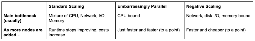
In any distributed computing system (even beyond Apache Spark), there exist well known scaling trends (runtime vs. number of nodes), as illustrated in the images below. These trends are universal and fundamental to computer science, so even if you’re running Tensorflow, OpenFOAM (computational fluid dynamics solver), or MonteCarlo simulations on many nodes, they will all follow one of the three scaling trends below:

Standard Scaling: As more and more nodes are added, the runtime of the job decreases, but the cost also increases. The reason is because adding more nodes is not free computationally, there are usually additional overheads to runtime such as being network bound (e.g. shuffles in Spark), compute bound, I/O bound, or memory bound. As an example, doubling the number of nodes to run your job results in a runtime of more than half of the original runtime if they exhibit standard scaling.
At some point, adding more nodes has diminishing returns and the job stops running faster, but obviously cloud costs start rising (since more nodes are being added). We can see point B here is running on let’s say, 5 nodes, but point A is running on 25 nodes. Running your job at point A is significantly less cost efficient and you may be wasting your money.
Embarrassingly Parallel: This is the case when adding more nodes actually does linearly decrease your runtime, and as a result we see a “flat” cost curve. This is traditionally known in the industry as “embarrassingly parallel” because there are no penalties for adding more nodes. This is usually because there is very little communication between nodes (e.g. no shuffles in Spark), and each node just acts independently.
For example at point B we are running at 5 nodes, but point A we’re running at 25 nodes. Turns out, although your number of nodes from A to B went up by 5x, your runtime also went down by 5x. So they both cancel out and you basically have a flat cost curve. In this case, you are free to increase your cluster size, and decrease your runtime for no extra cost! Due to the computational overheads mentioned above though, this case is quite rare and will eventually stop at large enough nodes (when exactly depends on your code).
Negative Scaling: This is the interesting case when running with more nodes is both cheaper and faster (the complete opposite of “Standard Scaling”). The reason here is that some overheads could actually decrease with larger cluster sizes. For example, there could be a network or disk I/O bound issue (e.g. fetch time waiting for data), where having more nodes increases the effective network or I/O bandwidth and makes your jobs run a lot faster. If you have too few nodes, then network or I/O will be your bottleneck as your Spark application gets hung up on fetching data. Memory bound jobs could also exhibit this behavior if the cluster is too small and doesn’t have enough memory, and there exists significant memory overhead.
For example at point B, we are running at 5 nodes, but now we only have 5 machines performing data read/write. But at point A we have 25 nodes, we have 5x more bandwidth on read/write, and thus the job runs much faster.
Real Customer Plots
The 3 scaling trends are universal behaviors of any distributed compute system, Apache Spark applications included. These scaling curves exist whether you’re running open source Spark, EMR, or Databricks — this is fundamental computer science stuff here.
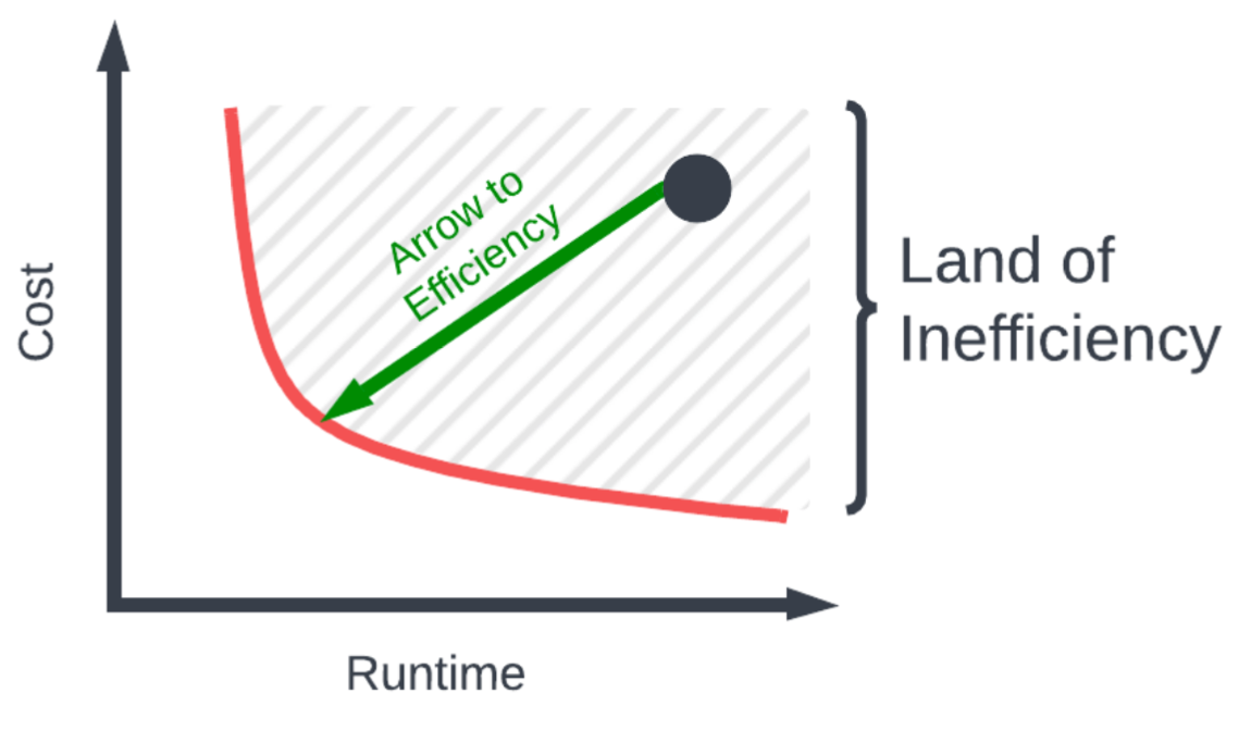
When we actually started processing customer logs, we noticed that the jobs weren’t even on the proper scaling curve, due to the improper configurations of Spark. As a result, we saw that customers were actually located in the “Land of Inefficiency” (as shown by the striped region below), in which they were observing both larger costs and runtime, for no good reason.
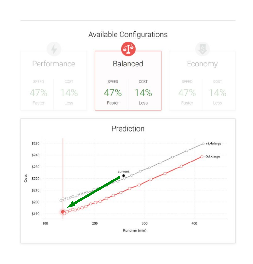
For example if you set your workers and memory settings improperly, the result you’d see in the gradient is a black “current” dot in the “Land of Inefficiency.” The entire goal of the gradient is to provide an easy and automatic way for customers to achieve an efficient Spark cluster.
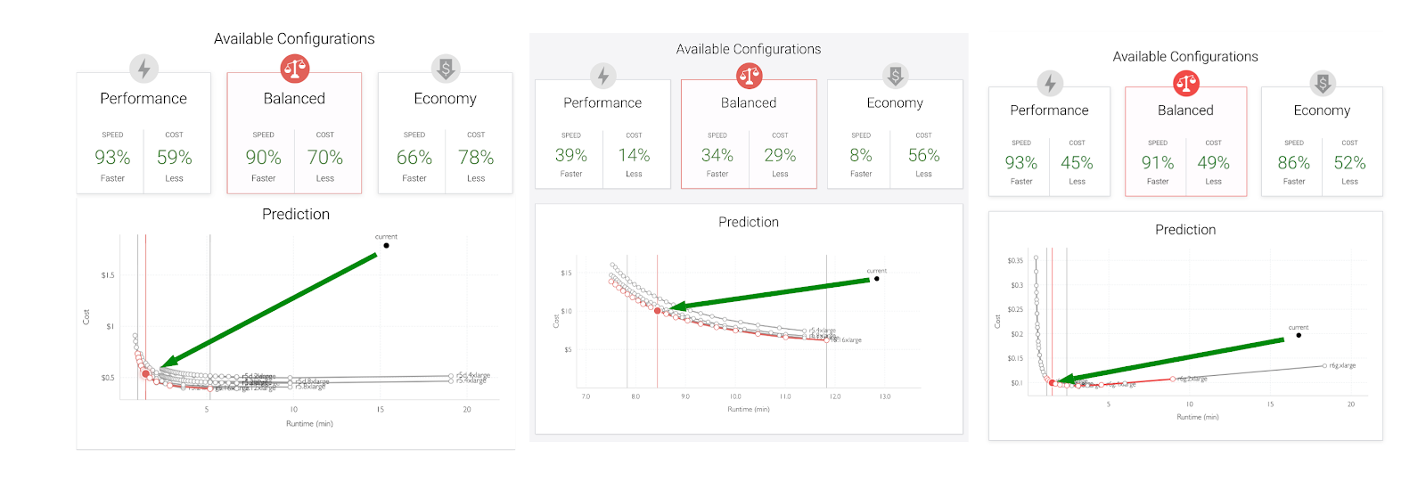
Standard Scaling — In the 3 screen shots below, we see the classic standard scaling for customer jobs. We see the classic “elbow” curve as described above. We can see that here in all 3 cases, all of the users were in the “Land of Inefficiency.” Some of the runtime and cost savings went up to 90%, which was amazing to see. Users can also tune the cost/runtime, based on their company’s goals.
Embarrassingly Parallel: In the screen shots below, we see almost flat curves for these jobs. In these cases the jobs were almost entirely CPU bound, meaning there was little communication between nodes. As a result, adding more nodes linearly increased the runtime. In this case, the jobs were still in the “Land of Inefficiency”, so substantial cost/runtime savings could still be achieved.
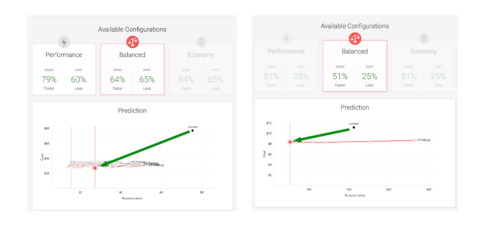
Negative Scaling — In the screen shots below, we see the negative scaling behavior. The issue here is a large amount of fetch wait time (e.g. network I/O) that causes larger clusters to be substantially more efficient than smaller clusters. As a result, going to larger clusters will be more advantageous for both cost and runtime.
Conclusion
We hope this was a useful blog for data engineers. As readers hopefully see, the scaling of your big data jobs is not straightforward, and is highly dependent on the particularities of your job. The big question is always, what is the bottleneck of your job? Is it CPU, network, disk I/O, or memory bound? Or perhaps it is a combination of a few things. The truth is, “it depends” and requires workload specific optimization. The Gradient for Apache Spark is an easy way to understand your workload, bring you out of the “Land of Inefficiency”, and optimize your job depending on the type of scaling behavior it exhibits.
One question we get a lot is — what about multi-tenant situations when one cluster is running hundreds or thousands of jobs? How does the Gradient take into account other simultaneous jobs? This solutions requires another level of optimization, and one we recently published a paper on entitled “Global Optimization of Data Pipelines on the Cloud”
 McKinley Culbert
 Vinoo Ganesh